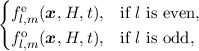
To numerically solve the set of equations presented in Section 3.1 they need to be discretized. In the course of this work the finite volume method (FVM) [35] has been used for the space spanned by the spatial coordinates and the total energy. Although it is possible to discretize the energy space by non-equidistant grids, equidistant grids are used here for simplicity. Upon discretization the expansion coefficients (cf. Equation (3.2)) are usually split into an even and odd part
| fl,m(x,H,t) = | (3.29) |
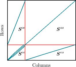
| Figure 3.2: | The sparsity pattern of the system matrix, where dashed red lines have been added to visualize the submatrices. The sparsity pattern of the system matrix with all terms excluding the time derivative assembled is shown. As can be seen, the submatrix Soo has no off-diagonals, since no odd unkown couples with another odd unkown. This allows to eliminate the odd-order unknowns from the equation system as demonstrated in [71]. |
When splitting the expanded BTE (cf. Equation (3.25)) into equations for odd and even unkowns an interesting pattern in the system matrix of the SHE equations emerges (cf. Figure 3.2). The system matrix for the BTE can be split into four submatrices, depending on the coupling they discribe. The matrix which contains couplings between even unkowns is See. The submatrix that couples even with odd unkowns is Seo and so forth. It is interesting to note that, since elastic and inelastic scattering operators only couple even unkowns with even unkowns, the submatrix Soo, which couples odd unkowns with odd unkowns, is a diagonal matrix. This allows for the use of the Schur-complement to compress the matrix to the size of the submatrix See [71]. This dramatically reduces the number of unkowns to be solved for to the size of See, which makes the system of equations much smaller. Thus the system is easier to solve on a common workstation using standard linear solvers and preconditioners such as incomplete LU factorization with threshold. The structure of the system matrix is shown in Figure 3.3 and clearly visualizes the dependence of the SHE equations via the H-grid on the electrostatic potential. At this point it has to be noted that the system matrix of the time-independent SHE expanded BTE exhibits an M-matrix property. An exhaustive explanation of the discretized set of equations can be found in [67].
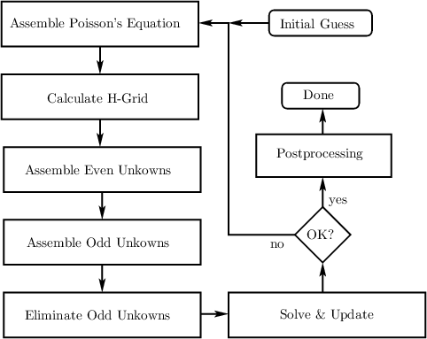
| Figure 3.3: | A flowchart of the SHE method. In every iteration Poissons equation is assembled first. After this the H-grid is built for the assembly of the equations for even and odd unkowns. Before solving the system of equations and reevaluating the potential and carrier concentrations, the size of the system matrix is reduced by elimination of odd-order unkowns [71]. This is repeated until changes in the potential are smaller than a given value. |