Time-dependent SHE of the BTE

3.6 Time-dependent SHE of the BTE

First results for a time-dependent SHE using the H-transform have been reported in [75]. However, the additional derivative,

∂_tf(x,E,t)	= +
	= ±∥q∥,	(3.38)

resulting from the H-transform was not considered in [75] and first reported in [49]. As stated, in a SHE of the BTE the H-transform is used to eliminate the derivative with respect to energy in the free streaming operator.

When applying the finite volume method in the energy space, the additional coupling terms read

	±∫ _{H_n^-}^H_n⁺∥q∥dH
	⇒±∥q∥∫ _{H_n^-}^H_n⁺dH
	= ±∥q∥,	(3.39)

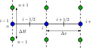
where the subscript i denotes the ith spatial grid point and n is the nth energy grid point (cf. Figure 3.7). The energy space is discretized using equidistant sampling points, that is H_n - H_n-1 = ΔH, where ΔH is the distance between two adjacent energy grid points. For integration H_n⁺ and H_n^- are used and defined as

H_n⁺	= (H_n + H_n+1)∕2,	(3.40)
H_n^-	= (H_n + H_n-1)∕2.	(3.41)

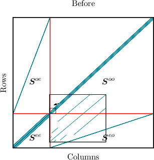
Although it is possible to discretize the energy space by non-equidistant grids here, we use equidistant grids for simplicity. The additional term on the right hand side of Equation (3.39) couples neighboring energies for even and odd-order unknowns in the system matrix S

(3.42)

where f^e∕o are the even and odd unkowns respectively, b^e∕o is the right hand side for even and odd unkowns, S^ee is the upper left sub-matrix coupling even unknowns to even unknowns, and S^oo is the lower right sub-matrix coupling odd-order unknowns with odd-order unknowns, and so forth. In a SHE of the stationary BTE the sub-matrix S^oo is a diagonal matrix. This makes it possible to reduce the number of unknowns considerably using the Schur-complement (S^ee -S^eo(S^oo)^-1S^oe)x^e = b^e -S^eo(S^oo)^-1b^o as shown in [71]. When assembling the time derivative the coupling of energies introduced by Equation (3.39) for even-order unknowns appearing in S^ee is similar to any coupling an elastic scattering operator would introduce. But the coupling of the energies for the odd-order unknowns from Equation (3.39), showing up in S^oo, destroys the diagonal sub-matrix structure of S^oo. This in turn increases the effort to eliminate the odd-order unknowns [71], since one has to carry out multiple line operations to restore the diagonal structure of S^oo in order to reduce the number of unknowns as it is done in a SHE for the time independent BTE (cf. Figure 3.5).

Figure 3.5:

The sparsity pattern of the system matrix before and after diagonalizing S^oo, where dashed red lines have been added to visualize the submatrices. On the left hand side the sparsity pattern of the system matrix with all terms (left figure), including the time derivative, assembled is shown. As can be seen the submatrix S^oo has non-zero offdiagonals, which prohibit the elimination of the odd-order unknowns. Through simple line operations the system matrix can be transformed such that S^oo is a diagonal matrix again. This allows to eliminate the odd-order unknowns from the equation system as demonstrated in [71].

To account for the time derivative of the expansion coefficients in the expanded BTE, we first assemble the stationary BTE and include Equation (3.39). Thus, the additional derivative for the total energy H in Equation (3.38) is accounted for. Now, assuming a known solution f_k of the SHE equations at time t_k, the fully assembled SHE equations for the next time t_k+1 = t_k + Δt without ∂_tf^n∕p are given as

S_k+1^jf_k+1^j = b_k+1^j,

(3.43)

where j denotes the jth iteration of the non-linear solver (e.g. Newton-Raphson). In order to assemble the time derivative for t_k+1, we use the implicit Euler scheme, although other more complex higher-order methods are available [76]. After a few algebraic transformations this yields

Δt

= Δtb_k+1^j + f_k,

(3.44)

where I is the unit matrix. Thus, one can assemble the system of SHE-BTE equations in each iteration of any non-linear solver as before and then include the time derivative by simple algebraic manipulations of the assembled stationary system of equations.

3.6.1 Comparison to Drift Diffusion

A comparison of the time derivative in the BTE and in the drift diffusion equations can be made by reproducing and exploring the origins of plasma oscillations. In this section the mathematical coherences between plasma oscillations as described by the BTE and by the drift diffusion model are compared.

Oscillations of the whole electron plasma in a semiconductor occur when electrons are shifted out of their equilibrium position around the fixed ions. Upon relaxation back into their respective equilibrium positions, the electrons oscillate around their equilibrium position. The characteristic frequency of plasma oscillations in a semiconductor is

ω_p =

where n is the carrier concentration, m_e is the electron mass and in this section here κ is used to denote the dielectric constant. For silicon ω_p is usually on the order of 1THz. We expect to see a peak in the real part of the admittance of a semiconductor device at the plasma frequency [36]. In the following we will use this fact to asses various assumptions for simulations using SHE and a stability analysis and show why the plasma frequency is important to test these assumptions. As stated, upon solving the time-dependent BTE using SHE and the H-transform one has to include an additional term in the time derivative (cf. Equation (3.38)) due to the H-transform. This term couples neighboring energies for even and odd-order unknowns. In particular, the coupling of the energies for the odd-order unknowns destroys the diagonal sub-matrix structure. One possible way to solve this is to diagonalize the sub-matrix for odd-order unknowns by a suitable algorithm before applying the algorithm from [71]. Nevertheless, this transformation renders a required stability analysis intractable. Another possibility to solve this problem is to assume that the potential change over time (cf. Equation (3.38)) as well as the gradient of the distribution function over energy are sufficiently small, effectively eliminating the couplings of the energies for the even and odd-order unknowns. As will be shown, a physically sound way to solve the problem of additional couplings for odd-order unknowns is to assume that the time derivative in the equations for the odd-order unknowns is sufficiently small. More precisely,

Δt^-1

(f_i,k+1^o(H_n+1) - f_i,k+1^o(H_n-1)) ≃ 0.

In order to assess the physical meaning of the above assumption we take a look at the drift diffusion model and show that neglecting the time derivative for odd-order unknowns is equivalent to neglecting the acceleration term

τ_m∂_tJ

(3.45)

in the drift diffusion model, where J is the current density and τ_m is the moment relaxation time. This assumption is equal to neglecting plasma oscillations and was shown to be valid for frequencies up to the plasma frequency [36]. For the drift diffusion model only the first two moments of the BTE are used, where closure is obtained by assuming equivalence of carrier temperature T_n and lattice temperature T_L. The moments of the distribution function are calculated using

⟨ψ_j⟩ = ∫ ψ_jfd³k = w_j ∫ k^jfd³k,

(3.46)

where j is the jth moment, ψ_j denotes the jth weight function and p_j is the jth prefactor. To obtain equations for the moments of the BTE, such as the drift diffusion model, the BTE is multiplied by increasing integer exponent of the wave vector k and a scalar prefactor w and afterwards integrated over the Brillouin zone. The first two moments of the BTE read

ψ₀	= 1 ⇒⟨ψ₀⟩ = ∫ fd³k = n
ψ₁	= ℏk ⇒⟨ψ₁⟩ = ℏ ∫ kfd³k
	= ℏ₌₀ + ∫ kf^od³k = J∕q,

where n is the electron density. The integral over the even part cancels out due to the symmetry of the first Brillouin zone. Thus, the current density is associated with the odd part or asymmetry of the distribution function. Applying the method of moments, assuming parabolic bands, and approximating the scattering operator Q{f} using the relaxation time approximation (RTA), one obtains the drift diffusion model [22]. Repeated from chapter 2 Section 2.3.1, the drift diffusion model with acceleration term, excluding Poisson’s equation, reads

ψ₀ ⇒	∂_tn -∥q∥^-1∇⋅J_n = -R,	(3.47)
ψ₁ ⇒	τ_m∂_tJ_n -∥q∥τ_mkB∇⋅ + m^*J_n = 0,	(3.48)
with	∂_tJ_n = ∫ k∂_tfd³k = ∂_t ∫ kf^od³k	(3.49)

with the mobility μ_n = ∥q∥τ_m∕m^*, R the scalar recombination term from Rⁿ{fⁿ,f^p}, m^* is the effective mass and kB the Boltzmann constant. As derived above the current density is associated with the odd part of the distribution function and thus also with the odd expansion orders in a spherical harmonics expansion. Thus neglecting the acceleration term in the DD model is equivalent to neglecting the time derivative of the odd part of the distribution function.

3.6.2 Stability

Even if the time derivative has been correctly implemented, numerical stability issues might still araise and lead to numeric artifacts in the simulation results [77]. At least a guideline, for how small Δx for spatial, ΔH for energy space and Δt for temporal discretization have to be in order to avoid any numeric artifacts, is required. To investigate the numerical stability of the time-dependent SHE-BTE a von Neumann analysis for electrons is carried out. The analysis for holes is done in the same way, yielding the same results and thus not shown here. Since the full numeric system is too complex and analytically intractable, we need to simplify matters. Thus, in the following we neglect plasma oscillations in the calculations to avoid the time derivative of the odd unknowns in the SHE. To keep the equations in the stability analysis as simple as possible, the finite volume method (FVM) in the 1D case under bulk conditions for silicon (cf. Figure 3.7) is used. Thus the force F, the generalized density of states Z as well as the group velocity v(k) are assumed to be spatially constant. To avoid notational clutter we use a superscript (o) to mark odd-order unknowns, indices and variables. The same is done for even-order unkowns (superscript e). We also drop the indices l,m, l′,m′ including the summation over these indices as well as the arguments to the distribution function. Additionally, we consider only elastic, velocity randomizing scattering processes and neglect the Pauli principle to further simplify the analysis. To summarize, we condense the scattering operator to

(

_{in-scattering} -

_{out-scattering}) =

{
ce, for even-orders
co, for odd orders,

where Y _0,0 is the first spherical harmonic, s is the scattering rate. Inelastic processes are not considered in the stability analysis. This assumption is needed to decouple the equations with respect to the total energy, which in turn leads to a tractable number of equations. Following [66, 47] the expanded and discretized BTE in a single spatial dimension (cf. Figure 3.7) for odd expansion orders reads

_≃0	+ + = c^of_i+1∕2,k+1^o,
_≃0	+ + = c^of_i-1∕2,k+1^o,

where f_i,k^e is the even unknown expansion coefficient for l,m at vertex i in the kth time step and f_i,k^o is the same for odd unknowns for l^′,m^′. Note that in the equations above we have neglected the acceleration term by setting the time derivative for odd unknowns to zero. For even-orders the expanded BTE in 1D reads

	Δt^-1-_=γ_{≃f_i,k+1^ex}
	+ f_i+1∕2,k+1^o -f_i-1∕2,k+1^o -f_i-1∕2,k+1^o -f_i+1∕2,k+1^o = c^ef_i,k+1^e.

Here it was assumed that f_i,k+1^e(H_n±1) can be written as f_i,k+1^eχ^± and χ = χ⁺ -χ^-, where χ^± are measures of how strong the distribution function increases/decreases over energy. In the above equations the shorthands

A^e∕o,± = ∫ _{H_n^-}^H_n⁺j_l,m^l′,m′(x_i±1∕2,H_n)dH,		(3.50)
B^e∕o,± = ∫ _{H_n^-}^H_n⁺A_l,m^l′,m′(x_i±1∕2,H_n)dH,		(3.51)

have been used for even and odd-orders, where A and j are the shorthands from Equation (3.26) for integrals over spherical harmonics. In this discretization A^e∕o,± accounts for the projected diffusion term in the free streaming operator of the BTE, whereas B^e∕o,± is the projected drift term and thus dependent on the driving force (electric field). Since we are assuming a homogeneous material and a constant driving force, we have A^e,+ = A^e,-, B^e,+ = B^e,-, A^o,+ = A^o,- and B^o,+ = B^o,-. With the simplified system given above, a von Neumann stability analysis is possible. For this we
(i) eliminate the odd unknowns in the equation for the even unknowns,
(ii) Fourier transform the obtained equation in space to transform spatial offsets into phase factors and
(iii) express the gain G as a function of Δx and Δt.
The Fourier transforms, where j is the imaginary unit, of f_i,k^e and f_i,k^o read G^kF^e exp (- jiθ)

and G^kF^o exp (- jiθ)

respectively, where G is the gain. Thus one obtains, after a few algebraic transformations, the gain

|G|² =

s - (aobe + aebo) cos(θ) + (aebo - aobe) sin(θ))2
------------------------2------------------
(y - z)

(3.52)

where

s =	c^oc^oΔt^-2(a^ea^o + b^eb^o + c^o(c^e - Δt^-1 + γχΔt^-1)
y =	a^o2b^e2 + a^e2(a^o2 + b^o2)
	+ 2a^ea^o(b^eb^o + c^o(c^e - Δt^-1 + γχΔt^-1))
	+ (b^eb^o + c^o(c^e - Δt^-1 + Δt^-1γχ))²,
z =	2(a^ob^e + a^eb^o)(a^ea^o + b^eb^o + c^o(c^e - Δt^-1 + γχΔt^-1))
	cos(θ) + 2a^ea^ob^eb^o cos(θ),

and

a^e = + ,	a^o = + ,	(3.53)
b^e = -,	b^o = -.	(3.54)

In order to have numeric stability of the time-discretized SHE-BTE in the von Neumann sense [78], the following relation must be fulfilled

≤ 1 ⇔

² ≤ 1,

(3.55)

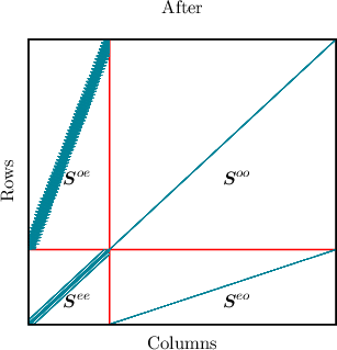
which states that any frequencies propagated by the BTE must not be amplified. For the lowest expansion order L = 1 the stability condition reduces to Δt > 0, since for the lowest order we have c = 0 and B = B^′ = 0 due to the H-transform. For L > 1, the stability condition reduces to

o Δt ≤ ---------c-(2---γχ)----------, if γχ < 2, (3.56) ao(ae - ae)+ bo (be - ae)+ ceco Δt > 0, otherwise, (3.57)

provided that

c^e > 0and

c^o < 0.

(3.58)

These conditions are naturally fulfilled due to the M-matrix property of the SHE equations for the lowest expansion order L = 1. In the limit of no driving force,

B^e± = 0and

B^o± = 0andγ = 0,

(3.59)

or sufficiently small driving force

|B^e±|≪

and

|B^o±|≪

(3.60)

the stability condition reduces to

Δt

(3.61)

where c^e is usually of the order of the density of states. Even though the above relation has been derived using a number of simplifying assumptions, it can be used as a rough guideline to choose Δt.

3.6.3 Energy Grid Interpolation

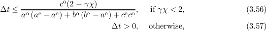
Aside from the usual stability concerns regarding hyperbolic partial differential equations discretized using the finite volume method, the H-transform poses another restriction to the maximum Δt. When considering the time-dependent BTE, the old solution f(x,H,t_k) from time step t_k has to be transferred from (x,H^k) to a new grid (x,H^k+1) (cf. Figure 3.6).

Figure 3.6:

The transfer of the old distribution function at time t_k from (x,H^k) (top graph) to a new grid (x,H^k+1) (bottom graph) during the iterations of the non-linear solver. If the change in the electrostatic potential φ is larger than ΔH∕∥q∥ there are grid points (red dots) in the new grid (red grid lines)

Convergence problems and numerical artifacts arise whenever a value of the old distribution function on (x,H^k) cannot be transferred/interpolated to a point on the new grid (x,H^k+1), because there is no value of the old distribution function available at that particular energy. This problem is always present, whenever the potential from time t_k to t_k+1 = t_k + Δt changes by more than

ΔH ----≥ Δφ, ∥q∥

(3.62)

where ΔH has to be carefully chosen. One can now either choose ΔH large enough to accommodate a predicted potential change Δφ within a time step and accept the inaccuracies in the distribution function introduced by this choice, or choose the boundary conditions for the Poisson equation and the subsequent time steps carefully in order not to violate Equation (3.62). This is very unsatisfying, since it is for example not possible to apply step functions as boundary conditions, with steps larger than Δφ. However, in case one is interested in the small signal response, a linearization of the free streaming operator of the BTE around the bias point [47] should be used instead of the time-dependent BTE to avoid the condition in Equation (3.62).

Even if the condition in Equation (3.62) is not violated, the distribution function f(x,H^k,t_k) needs to be transferred to the new grid such that the macroscopic quantities, that is charge carrier concentration and charge carrier current, are not modified by the interpolation of f from (x,H^k) to (x,H^k+1). Thus, the charge carrier density and current density are not modified by the interpolation of f from (x,H^k) to (x,H^k+1). Since the even part of the distribution function completely defines the charge carrier concentration and the odd part defines the charge carrier current, the even part is transferred such that

fe(x,Hk, tk)Z (Hk ) = f e(x,Hk+1, tk)Z(Hk+1 )

(3.63)

holds for the conservation of the carrier density. Likewise the new odd part f^o(x,H^k+1,t_k+1) is independently renormalized such that

f o(x, Hk,tk)Z (Hk )vg(Hk ) = f o(x, Hk+1,tk)Z (Hk+1 )vg(Hk+1 )

(3.64)

is fullfilled, in order to keep the current density constant. However, interpolation errors will occur during the transfer of the old solution onto the new H-grid, even if the condition in Equation (3.62) is fulfilled. Since the band edge is shifted by the potential during a single timestep, the first energy grid point (H^k = 0) closest to the band edge will be shifted under the new band edge or a grid point below the old band edge (H^k = -1) will be shifted above the new band edge. In the first case a sample point for the distribution function is lost. In the second case a new energy grid point for which there is no old distribution function available will be obtained. This effect cannot be mitigated when the H-transform is employed. The error introduced by this is quantified by

ˆe∕o k+1 k+1 f---(x,-H----,tk)Z-(H----). Δt

(3.65)

3.6.4 Probable Violation of Gauss’ Law

As stated in the previous section, it is currently not possible to avoid errors during energy grid interpolation. To better understand the implications of this, the discretized SHE-BTE equations per energy grid point, for a three-point stencil are investigated. In Figure 3.7 a homogeneous, uniformly discretized three-point stencil for a single spatial dimension is shown. The system of equations for this simple three point stencil will be derived and evaluated in the following. Assuming that the even unkowns on the left and right point of this three point stencil are fixed by dirichlet boundary conditions, only the even expansion coefficient f_l,m^e in the center and the two odd unkowns on the two edges f_l,m^o need to be determined. To simplify matters, a first-order expansion (L = 1) and elastic scattering is assumed. Thus we are left with three unkowns, the even unkown f_0,0ⁱ, the odd unknown on the left edge f_1,0^i-1∕2 and the odd unknown f_1,0^i+1∕2 on the right edge. For these unkowns the equations of any point on the H-grid read

V Zⁱ∂_tf_0,0ⁱ -v^i-1∕2Z^i-1∕2f_1,0^i-1∕2 + v^i+1∕2Z^i+1∕2f_1,0^i+1∕2 =	0,	(3.66)
V Z^i-1∕2∂_tf_1,0^i-1∕2 -v^i-1∕2Z^i-1∕2f_0,0^i-1 + v^i-1∕2Z^i-1∕2f_0,0ⁱ =	Sf_1,0^i-1∕2V,	(3.67)
V Z^i+1∕2∂_tf_1,0^i+1∕2 -v^i+1∕2Z^i+1∕2f_0,0ⁱ + v^i+1∕2Z^i+1∕2f_0,0ⁱ⁺¹ =	Sf_1,0^i+1∕2V,	(3.68)

where V is the box volume, Z is the generalized density of states, v is the group velocity, S is the elastic scattering term and the interface area A between two points connected by an edge is assumed to be equal to unity. Introducing a = (AΔx)∕(2V ), neglecting the time derivatives of the odd-order unkowns for the sake of argument and using a Backward-Euler scheme one obtains

	-_{Energy grid interpolation error}
	+ q
	-_A
	+ _B = 0,	(3.69)

where the quantities form the previous timestep are highlighted by the superscript old and the energy grid interpolation error has been considered. Since it will be important when considering the time derivative, it is shown how to obtain the familiar charge conservation law (Gauss Law). Integration of the above equation over energy from H = 0 to infinity yields term by term,

∂_tn_i - (D₁ + D₂)

_i + 0 + D₂n_i+1 + 2(D₁ + D₂)n_i - D₁n_i-1 = 0,

(3.70)

where D are transport coefficients and

∫ ₀^∞dH	= _i,	(3.71)
q ∫ ₀^∞dH	= 0.	(3.72)

If there is no interpolation error at all, i.e.

_i = 0, one would obtain the familiar charge conversation law

∂_tnⁱ - D₁n^i-1 + (D₁ + D₂)nⁱ - D₂nⁱ⁺¹ = 0,

(3.73)

instead. From this it is clear that any energy grid interpolation error leads to artifacts (

) in the charge carrier density.

Figure 3.7:

Illustration of a staggered three point stencil in a single spatial dimension. The even unknowns are assembled on the vertices (blue circles), whereas the odd unknowns are assembled on the edges. Additionally for each vertex there is an equidistant grid (green circles) for the total energy of the charge carriers over which the distribution function is resolved.

3.6.5 The Shockley-Haynes Experiment

To assess the derived results we added the time derivative of the BTE to the open source simulator ViennaSHE [65]. In the first numerical experiment, similar to the famous Shockley-Haynes experiment in [79], the drift and diffusion of minority carriers in a p-type silicon resistor 5μm long under carrier-phonon and impurity scattering were investigated. The Shockley-Haynes experiment was selected, since throughout the whole simulation the potential and thus the H-grid remain virtually unchanged, provided that the distortion in the carrier concentration remains small. Assuming symmetry in two axis, the simulation was carried out in a single dimension using a Δx of 10nm. Additionally, to have the low-field conditions required for the estimation of the low-field mobility, we chose an uniform electric field of 0.5kV∕cm.

Figure 3.8:

A schematic of the 1D domain used. In this experiment a Gaussian disturbance in the electron density was introduced close to the left terminal (LT) by raising the energy distribution function uniformly over energy. The carriers then drift, caused by the electric field, towards the right terminal (RT) and diffuse in all directions.

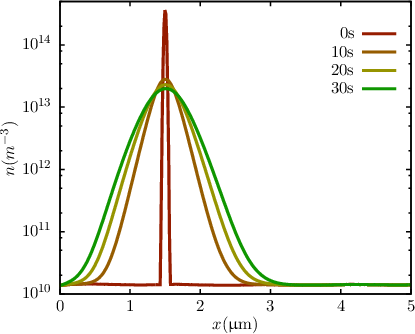
In this initial configuration we artificially introduced, at time zero, a Gaussian disturbance in the electron density (cf. Figure 3.8), such that changes in the electric field over time can be safely neglected. This was accomplished by uniformly raising the electron distribution function over the energy such to reach the desired electron density. Then a time-dependent simulation with a stepping of Δt = 10ps was carried out. 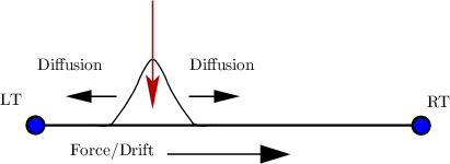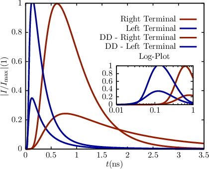Since changes in the electric field have been kept neglected, the displacement current was neglected too. In the first few hundred picoseconds the high energy carriers diffuse strongly. Thus, at first most electrons diffuse out of the left terminal before being accelerated towards the right terminal by the small electric field (cf. Figure 3.9). To see most of the diffusion in the current, the disturbance has been placed close to the left terminal (cf. Figure 3.10). After 700ps the carrier drift dominates and the current through the right terminal peaks. One can also calculate the low field mobility from this experiment by observing the velocity of the electron peak towards the right contact. In the presented experiment we obtained an electron mobility of 1430cm∕Vs with an uncertainty of ±20cm∕Vs due to the discretization.

Figure 3.9:

The electron current over time in a p-type resistor (cf. Figure 3.8) for the left (LT) and the right terminal (RT). In good approximation it can be said that the current at the left terminal corresponds to the diffusion and the current at the right terminal corresponds to the drift of the electrons. It is also noticeable that the electron current at the left terminal is higher for drift diffusion compared to a SHE solution of the BTE.

Figure 3.10:

The electron concentration in a p-type resistor for various times. At time t = 0s a Gaussian disturbance is introduced and observed over time. In the first few time steps (Δt = 10ps) the carriers strongly diffuse, before gaining enough momentum towards the right terminal (5μm).

[next] [prev] [prev-tail] [front] [up]