4.3 The First-Oder Quantum Corrected SHE of the BTE
The density gradient model has been previously successfully introduced into a full-band Monte Carlo
simulator [84]. Introducing quantum correction potentials in a SHE of the BTE influences the step in
which the H-grid is calculated, shown in Figure 3.3, quite strongly. First the discretization of the
H-space needs to be split for electrons and holes, since different correction potentials are applied for
electrons and holes respectively. When evaluating the recombination terms (cf. Section 3.5), care must
be taken to only use the distribution function directly or the charge carrier concentrations, but not the
quantum corrected electrostatic potential in order to avoid mistakes. Incorporating the quantum
correction potentials
| γn | =  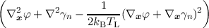 , , | (4.12)
|
| γp | =  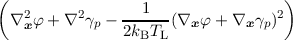 , , | (4.13) |
for electrons and holes respectively leads to a modified H-transform
![{
ϵ- ∥q∥[φ (x,t)+ γn(x,t)], for electrons
H = ϵ+ ∥q∥[φ (x,t)+ γ (x,t)], for holes,
p](diss232x.png) | (4.14) |
where the force F is calculated per charge carrier using
| Fn(x,t) | = -∇x(±EC ∓∥q∥![[φ (x, t) + γn(x,t)]](diss233x.png) ), ), | (4.15)
|
| Fp(x,t) | = -∇x(±EV ∓∥q∥![[φ (x, t)+ γp(x,t)]](diss234x.png) ). ). | (4.16) |