3.4.3 Jump-and-Walk

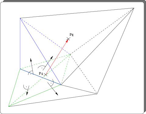
This technique uses a very simple algorithm to find the element surrounding a given point. The algorithm is structured into two parts. The first part selects a start tetrahedron. The second part is an iterative search. Beginning with the start tetrahedron, the algorithm chooses neighboring tetrahedrons such that the distance to the search point is reduced. To choose among the $4$ neighboring tetrahedrons, the dot products of the normal vectors of the bounding triangles and the vector from the search to the in-sphere point of the start tetrahedron are computed. The algorithm is then repeated until either the tetrahedron containing the search point was found, or a boundary face was reached in which case the algorithm has to start at another starting tetrahedron. Fig. 3.15 depicts the principle of this algorithm.

Figure 3.15: Jump and walk algorithm. $P_S$ denotes the in-sphere point of the start tetrahedron, $P_E$ is the point to search (end point). To determine which neighboring tetrahedron lies closest to $P_E$, the dot products of the vector from $P_S$ to $P_E$ and the normal vectors of all bounding triangles are computed. The triangle whose normal vector results in the largest dot product is chosen, and the adjoining tetrahedron (blue) is taken as the next step towards the search point.

The big advantage of this algorithm is its vanishing pre-processing time. The imposed memory overhead is also considerably smaller compared to the oct-tree. The only requirement to the data structures holding the grid elements is that information about neighboring elements needs to be computed and held in memory. In the following we compare oct-tree and jump-and-walk on the basis of the above example (management of $\approx 2\cdot 10^6$ elements). If, for the sake of simplicity, the implementation of the algorithm does not distinguish between boundary and inner triangles, each triangle holds two handles to tetrahedrons and three point handles. We estimate the number of triangles to be $6\cdot 10^6$, so that the total amount of memory overhead computes to $\approx 240$ megabytes which is considerably more as with the oct-tree.

The average performance of the point location can not be estimated easily since it strongly depends on the selection of the starting element. Several algorithms to select such an element were proposed. One possible strategy is to randomly choose several points (of elements) and use an element that references the point with the smallest Euclidean distance. Another strategy accounts for locations that are (possibly) geometrically related to each other. The algorithm remembers the result of the last location and takes this as starting condition for the next. In literature the "theoretical performance" for jump-and-walk on a Delaunay triangulation is given as being proportional to $n^{1/d}$ (in dimension $d$) when the points are randomly distributed [50].

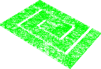
The performance also strongly depends on the shape of the geometry. If we look at the structure depicted in Fig. 3.16,

Figure 3.16: Disadvantageous two-dimensional grid for the jump-and-walk search algorithm.

the thin region between the two thicker ones is unfavorable for a jump-and-walk point location algorithm in case the query point is in the thin region. Fig. 3.17 depicts a disadvantageous three-dimensional case.

Figure 3.17: Disadvantageous three-dimensional grid for the jump-and-walk search algorithm.

The likelihood of picking a starting element within the thicker regions is proportional to the ratio of the number of points in the two regions and thus, can be very high if the algorithm randomly chooses points and computes Euclidean distances to the query point.

Two algorithms to select a starting tetrahedron were implemented. The first algorithm uses a configurable number of randomly chosen points and picks the one with the smallest Euclidean distance to the search point. From the set of tetrahedrons that reference this point the first is chosen as the start tetrahedron. The second selection algorithm uses a point bucket oct-tree to store all points of the mesh. A point that is close to the search point is chosen. The algorithm to find a close point takes advantage of the leaf structure of the point bucket oct-tree in the following manner. First the deepest node or leaf that contains at least one point is searched. If a leaf was found and the search point lies within the coordinates of this leaf then the point stored on the leaf is taken as start point. Otherwise the neighbors of the node (or leaf) are searched. This algorithm is guaranteed to return a point if the point bucket oct-tree is not empty. A tetrahedron is then chosen from the close point in the same way as with the first algorithm.

After the selection of the start tetrahedron the actual walk algorithm is started. The algorithm remembers all tetrahedrons that were already met to avoid endless loops. If the algorithm encounters the surface of the mesh, another starting tetrahedron is chosen.

The implementation of jump-and-walk is a general templatized code that supports point location for two-dimensional and three-dimensional grids respectively.

2003-03-27