|
|
|
|
Previous: 5.1 Introduction Up: 5.1 Introduction Next: 5.1.2 Calibration of Models |
|
|
|
|
Previous: 5.1 Introduction Up: 5.1 Introduction Next: 5.1.2 Calibration of Models |
Inverse Modeling
is a technique to adapt parameters of a physical model to a set of experimental
data (measurements) such that the error between the output of the model
(simulation) and the measurements is as small as possible. This is e.g. used to
calibrate mobility models of device simulators to measured ![]() ,
, ![]() ,
and
,
and ![]() curves of a transistor. Another challenging task of inverse modeling of
semiconductor devices is to extract the dopant concentration profile of a device
by means of a device simulator [84,85]. The device simulator thereby
serves as a "meter" to extract
curves of a transistor. Another challenging task of inverse modeling of
semiconductor devices is to extract the dopant concentration profile of a device
by means of a device simulator [84,85]. The device simulator thereby
serves as a "meter" to extract ![]() ,
, ![]() and
and ![]() curves of an
artificial device. The artificial device is characterized by a set of parameters
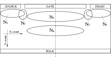
describing geometry features and dopant concentration. Fig. 5.2 depicts
such an artificial device with
curves of an
artificial device. The artificial device is characterized by a set of parameters
describing geometry features and dopant concentration. Fig. 5.2 depicts
such an artificial device with ![]() different doping "peaks" (
different doping "peaks" (![]() to
to
![]() ). The device is symmetric along the dash-dotted line. The peaks are
modeled as Pearson Type IV and
Gaussian distribution functions as described in [86].
). The device is symmetric along the dash-dotted line. The peaks are
modeled as Pearson Type IV and
Gaussian distribution functions as described in [86].
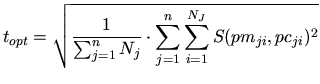
The extracted
operating points are then compared to measured ones. For ![]() curves with
dimensions
curves with
dimensions ![]() the target
the target ![]() delivered to the optimizer is given as the
component wise scaled quadratic deviation of the computed (
delivered to the optimizer is given as the
component wise scaled quadratic deviation of the computed (![]() ) from the
measured (
) from the
measured (![]() ) operating points:
) operating points:
with
In (5.2) and (5.3) the relative error is scaled
to values between ![]() . This is necessary to avoid a too large target value
for error vectors where the difference for some components is in the range of
several magnitudes. Once the optimizer is near an optimum the error vector is
comparably small. However, during the computation of the gradient or during the
evolution of a global optimizer intermediate parameter states will be generated
that are far away from the optimum. Since a simulator will not stop and produce
a result for an arbitrary given input, a large error vector is created by the
optimization framework to indicate a failed simulation. For global
optimizers, such an artificially large target encourages the optimizer to
discard the state. Such states simply become extinct. For a local optimizer an
artificial target value is the only way to continue in case of a simulation
failure, although the usefulness is questionable5.1.
. This is necessary to avoid a too large target value
for error vectors where the difference for some components is in the range of
several magnitudes. Once the optimizer is near an optimum the error vector is
comparably small. However, during the computation of the gradient or during the
evolution of a global optimizer intermediate parameter states will be generated
that are far away from the optimum. Since a simulator will not stop and produce
a result for an arbitrary given input, a large error vector is created by the
optimization framework to indicate a failed simulation. For global
optimizers, such an artificially large target encourages the optimizer to
discard the state. Such states simply become extinct. For a local optimizer an
artificial target value is the only way to continue in case of a simulation
failure, although the usefulness is questionable5.1.
|
|
|
|
Previous: 5.1 Introduction Up: 5.1 Introduction Next: 5.1.2 Calibration of Models |
![$\displaystyle S(a, b) = \left\{ \begin{array}{ll} 0 & \mbox{if $a = 0$\ and $b ...
...h{\left\vert b\right\vert}\right]}}} & \mbox{otherwise} \\ \end{array} \right.$](img148.png)