2.3 Galerkin's Method

A weak formulation of ( $\ref{gen_eq}$) for $\frac{\partial \mathbf{c} }{\partial t}=0$ is given by,

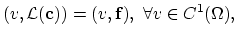$$(v,\mathcal{L}(\mathbf{c}))=(v,\mathbf{f}), \forall v\in C^{1}(\Omega),$$ (2.7)

$v$ is called test function. In this case we have an inner product between a scalar and a vector function on both sides of equation (2.7).

If the solution of the problem (2.1) in the space $\mathcal{V}$ exists, than it is possible to represent this solution as the sum of an infinite series with the weighted basis functions of the space $\mathcal{V}=C^2(\Omega)$.

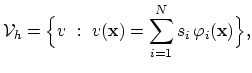
The central idea of Galerkin's method is to seek the solution of the problem given by (2.1), (2.2), and (2.3) not represented through the basis functions of the infinite space $\mathcal{V}$ but through the basis functions of the finite space $\mathcal{V}_h\subset \mathcal{V}$ ( dim$\mathcal{V}_h<\infty$) [9,10]. Such a solution can only be an approximation of the real solution of (2.1).
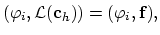
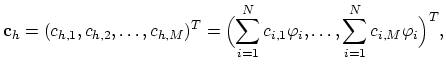
We choose $N$ linear independent functions $\varphi_i\in\mathcal{V}$, $i=1,\dots,N$ which span the space $\mathcal{V}_h$, e.g.

$$\mathcal{V}_h=\Bigl\{ v : v(\mathbf{x})=\sum_{i=1}^{N}s_i \varphi_i(\mathbf{x})\Bigr\},$$ (2.8)

where $s_i\in \Bbb{R}$.
Now we can write equation (2.7) in the space $\mathcal{V}_h$,

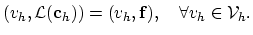$$(v_h,\mathcal{L}(\mathbf{c}_h))=(v_h,\mathbf{f}),\quad \forall v_h\in \mathcal{V}_h.$$ (2.9)

Trivially $\varphi_i\in\mathcal{V}_h$, and we can write,

$$(\varphi_i,\mathcal{L}(\mathbf{c}_h))=(\varphi_i,\mathbf{f}), i=1,\dots,N.$$ (2.10)

Considering that

$$\mathbf{c}_h=(c_{h,1},c_{h,2},\dots,c_{h,M})^T=\Bigl(\sum_{i=1}^{N}c_{i,1}\varphi_i,\dots,\sum_{i=1}^{N}c_{i,M}\varphi_i\Bigr)^T,$$ (2.11)

we see that inner product in (2.10) transforms the differential operator $\mathcal{L}$ into the operator

$$\ell : \Bbb{R}^{n}\rightarrow \Bbb{R}^{n}, n=M\cdot N,$$ (2.12)

and we write (2.10) as a system of nonlinear algebraic equations

$$\ell_{ij}(c_{1,1},\dots,c_{1,N},\dots,c_{M,1},\dots,c_{M,N})=(\varphi_i,f_j), i=1,\dots,N j=1,\dots,M.$$ (2.13)

This equation is solved by means of Newton's method (see Section 2.6). The solutions $c_{ij}$ of (2.13) are used to construct approximation of the functions $c_i(\mathbf{x})$ from $\mathcal{V}_h$ using (2.8).
The value

$$R_{ij}=\ell_{ij}(c_{1,1},\dots,c_{1,N},\dots,c_{M,1},\dots,c_{M,N})-(\varphi_i,f_j), i=1,\dots,N j=1,\dots,M$$ (2.14)

is called residuum.