Next: 2.6 Newton Methods
Up: 2. Finite Element Method
Previous: 2.4 Time Dependent Problems
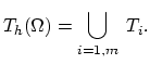
2.5 Finite Element Spaces and Meshes
The basic concepts of Galerkin's method, such as weak formulation of the problem and the transformation of this weak formulation from the functional space with infinite basis into the functional space with finite basis, as presented in Sections 2.3 and Sections 2.4, are presented here to introduce the finite element method.
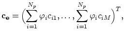
The construction of the finite element space
 begins with subdividing the domain
  into a set
 of non-overlapping elements
 . The domain can now be approximated with a mesh domain,
 |
(2.21) |
We denote as  the set of all points of the mesh domain
 .
Each point
.
Each point  has an unique global index
 , where
  is the number of all points in the mesh.
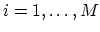
A point has several local indices.
is the number of all points in the mesh.
A point has several local indices.
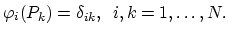
The basis functions
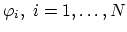 of the finite element space
fulfill,
of the finite element space
fulfill,
 |
(2.22) |
Since they are defined on nodes of the mesh, we call them basis nodal functions.
In the finite element praxis basis nodal functions are almost exclusively low order polynomials.
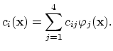
For further discussion it will be useful to have approximations of functions
 represented for each element
 with
with
 |
(2.23) |
 represents the local index of the element vertices and
  is the number of element vertices.
We use linear basis functions and tethraedrons
as elements. Therefore  , and each of the functions
  ,
,
 is approximated on the elements
  of the discretization
using the linear basis functions
of the discretization
using the linear basis functions
 ,
,
 |
(2.24) |
Now we can also define the operator
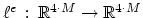 for each element of the discretization,
 |
(2.25) |
The inner product is calculated over the element . The local residuum vector is defined as,
 |
(2.26) |
Determining the operator  requires the calculation of the basic nodal functions,
 |
(2.27) |
The coefficients
 are functions of the nodal coordinates and
  is the volume of the element [11].
Constructing of frequently demands calculations of the following integral,
is the volume of the element [11].
Constructing of frequently demands calculations of the following integral,
 |
(2.28) |
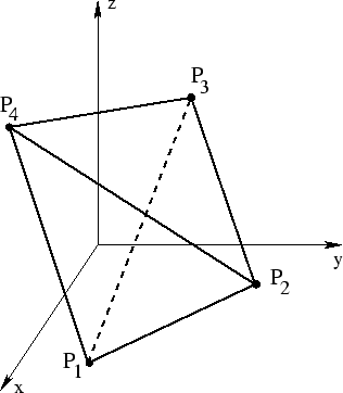
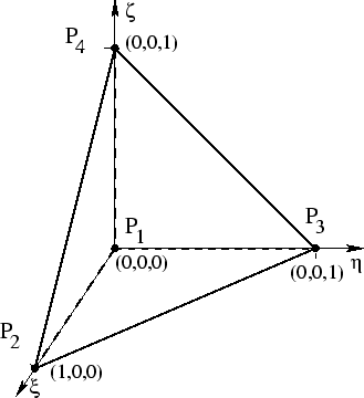
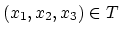
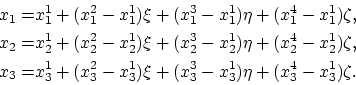
In this case (2.27) can be used, but instead it is more practical to project the discretization element (Figure 2.1) into normalized coordinate system element  (Figure 2.2). Each point
 is a bijective projection of the corresponding point
 ,
,
 |
(2.29) |
The basis nodal functions on are
 ,
,
 ,
,
 and
and
 .
(2.28) is now calculated as
.
(2.28) is now calculated as
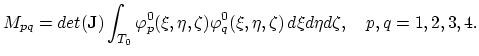 |
(2.30) |
 is the Jacobian of the projection (
 ),
),
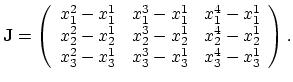 |
(2.31) |
Figure 2.1:
Tethraedal element in  -coordinate system
|
|
Figure 2.2:
Tethraedal element in normalized
 -coordinate system
|
|
Next: 2.6 Newton Methods
Up: 2. Finite Element Method
Previous: 2.4 Time Dependent Problems
H. Ceric: Numerical Techniques in Modern TCAD