
 ∫
-L∕2L∕2dse-i2qΔk⋅sδV
∫
-L∕2L∕2dse-i2qΔk⋅sδV 
 - V
- V  ,
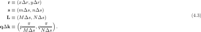
,The Wigner potential (WP) is of central importance in the signed-particle method as it dictates the particle generation statistics (see Section 3.7.5). This section summarizes the contributions made in this thesis related to the WP, aiming at an optimized computational implementation. First, the full discretization of the WP is shown, which introduces the computational task (Section 4.1.1). Thereafter, a highly efficient algorithm to calculate the two-dimensional (2D) WP is presented (Section 4.1.2), which is of importance in the pursuit of self-consistent solutions. Finally, the implications the choice of the coherence length has on physical and computational aspects is discussed (Section 4.1.3); a physically relevant example clearly illustrates how the encountered discretization effects can be mitigated.
The semi-discrete WP
| V W | ≡∫
-L∕2L∕2dse-i2qΔk⋅sδV | (4.1) |
| δV | ≡ V - V , | (4.2) |
The WP has to be computed at every mesh point in the domain for a given potential profile. The calculation of the 2D WP can consume considerable computation time, if it must be recalculated many times, e.g. if the potential is time-dependent or a self-consistent solution is pursued. This section presents an algorithm, first introduced in [128], named the box discrete Fourier transform (BDFT), which reduces the computational effort of calculating the 2D WP by at least a factor of five.
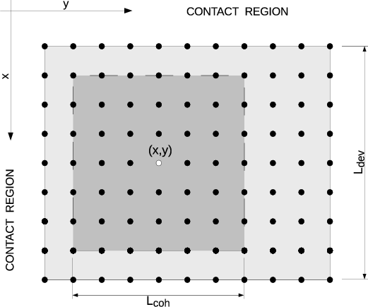
 , centred at node
  in the discretized domain, of size Ldev =
  , surrounded by
semi-infinite contact regions.
, surrounded by
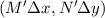
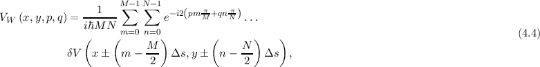
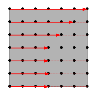
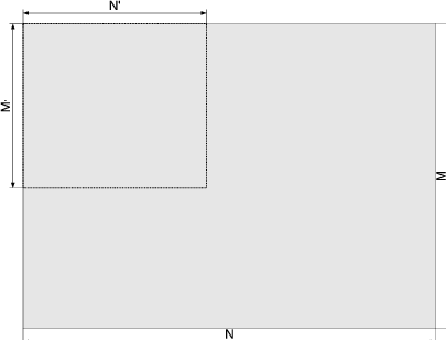
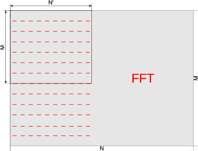
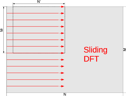
semi-infinite contact regions.Equation (4.4) is akin to a 2D DFT of (4.2), conventionally calculated using a row-column decomposition scheme, which entails the successive application of a one-dimensional (1D) DFT algorithm: With reference to Figure 4.2, consider a M′× N′ matrix of values representing the calculated potential differences, as per (4.2). First the 1D DFT of each row of values is calculated, which yields a M′× N′ matrix of Fourier coefficients. Thereafter, the 1D DFT of each column of the latter matrix is calculated, the result of which corresponds to the 2D DFT.
The fast Fourier transform (FFT) algorithm has a computational complexity, for a problem size N, of  (N log 2N) and presents the de facto standard
algorithm for calculating 1D DFTs, thanks to flexible, highly optimized implementations, which are freely available in libraries, like FFTW3 [129].
Algorithms which directly calculate multi-dimensional DFTs exist, e.g. [130, 131], and have a reduced computational complexity, which should
theoretically result in superior computational performance. However, these advantages are most often completely eroded in practical implementations,
which can be attributed to the fact that the cache complexity of algorithms implemented on modern hardware architectures plays an equally
important role as the computational complexity. Moreover, these multi-dimensional algorithms require extensive ’tailoring’, e.g. to the number of
dimensions or problem size
(N log 2N) and presents the de facto standard
algorithm for calculating 1D DFTs, thanks to flexible, highly optimized implementations, which are freely available in libraries, like FFTW3 [129].
Algorithms which directly calculate multi-dimensional DFTs exist, e.g. [130, 131], and have a reduced computational complexity, which should
theoretically result in superior computational performance. However, these advantages are most often completely eroded in practical implementations,
which can be attributed to the fact that the cache complexity of algorithms implemented on modern hardware architectures plays an equally
important role as the computational complexity. Moreover, these multi-dimensional algorithms require extensive ’tailoring’, e.g. to the number of
dimensions or problem size  , making general purpose implementations difficult, thereby hampering a wide-spread adoption of such algorithms.
The BDFT algorithm expands on the idea of the 1D sliding DFT [132, 133]: The sliding DFT calculates the Fourier coefficients of a sequence  using the
coefficients calculated for
using the
coefficients calculated for 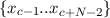 :
:
Each application of (4.5) consists of two real additions and two complex multiplications, which have to be repeated for each value of p. Therefore, the sliding DFT
has a computational complexity of (N). To apply the sliding DFT, as in (4.5), the two sequences under consideration must differ by only a single value; the
potential values of each row (column) of the coherence boxes associated with two horizontally (vertically) adjacent nodes in the domain also differ only by a single
value. This observation is exploited to calculate the 2D WP in an efficient manner.
Unlike the potential values, all the values of the potential difference (4.2) change between adjacent nodes. To allow a direct application of (4.5) to calculate (4.4), (4.1) is reformulated using a substitution of variables (Fourier shift theorem), such that
This formulation has the additional advantage that it avoids the calculation of the potential difference, saving further computation time. It can be noted that (4.5)
allows, unlike the FFT, to easily compute only selected momentum  values, which do not have to be uniformly spaced. This can be of interest
under certain physical considerations, e.g. uniformly spaced energy grid, and offers an additional possibility to reduce computational costs.
values, which do not have to be uniformly spaced. This can be of interest
under certain physical considerations, e.g. uniformly spaced energy grid, and offers an additional possibility to reduce computational costs.
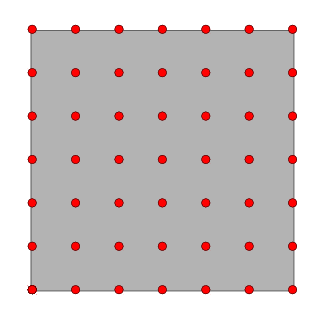
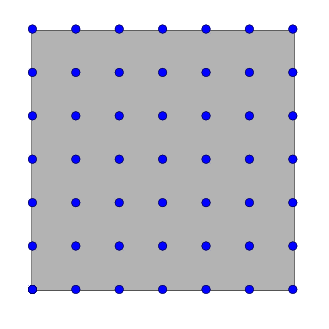
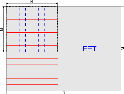
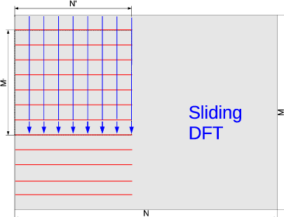
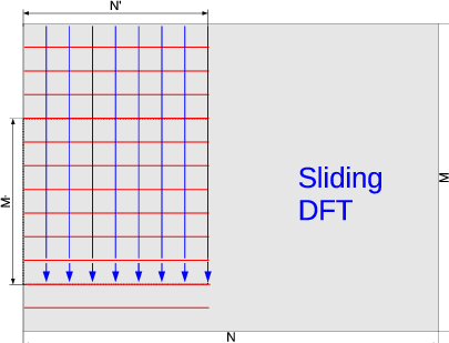
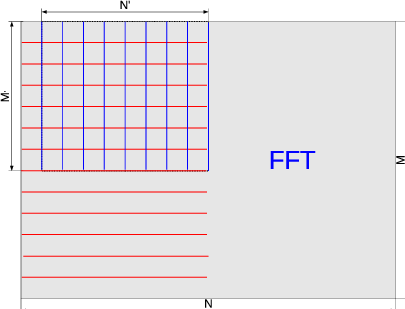
The BDFT algorithm is applied to calculate the WP at each node in the domain, using the following procedure (as visualized in Figure 4.3): First, the 1D DFT of
the first N′ potential values in each of the M rows in the domain are calculated, using an FFT algorithm (Figure 4.3(b)); the resulting Fourier coefficients are
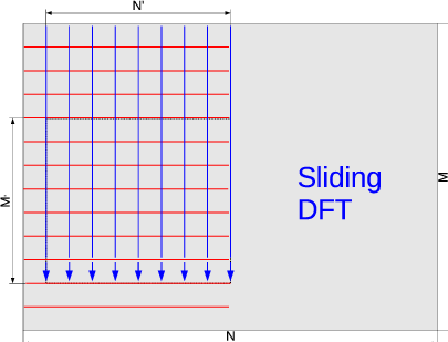
retained in an array of size N′× M. Thereafter, the 1D DFTs of the first M′ Fourier coefficients of each of the N′ columns are calculated (Figure 4.3(c)),
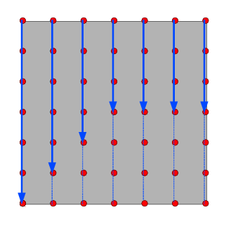
which yields an M′× N′ matrix of Fourier coefficients representing the WP for the top-left node, V W  . After this initialization, the
coherence box is moved downwards to the next node for which the WP is calculated by simply applying (4.5) to calculate the DFTs of the columns
(Figure 4.3(d),(e)). Once the WP has been calculated for each node in the first column of the domain, the N′× M array is developed to the right
(Figure 4.3(f)), again using (4.5). From there the same procedure as used for the first column (Figure 4.3(a)-(e)) is repeated for the second column of
nodes (Figure 4.3(g),(h)) etc., until the entire domain has been covered. Variations of the initialization approach can be envisioned, but the
presented procedure shows favourable serial performance and cache complexity; a parallelized implementation would require multiple (modified)
initializations.
. After this initialization, the
coherence box is moved downwards to the next node for which the WP is calculated by simply applying (4.5) to calculate the DFTs of the columns
(Figure 4.3(d),(e)). Once the WP has been calculated for each node in the first column of the domain, the N′× M array is developed to the right
(Figure 4.3(f)), again using (4.5). From there the same procedure as used for the first column (Figure 4.3(a)-(e)) is repeated for the second column of
nodes (Figure 4.3(g),(h)) etc., until the entire domain has been covered. Variations of the initialization approach can be envisioned, but the
presented procedure shows favourable serial performance and cache complexity; a parallelized implementation would require multiple (modified)
initializations.
The BDFT algorithm was benchmarked against an FFT implementation using the FFTW library [129], with a setup detailed in Table 4.1. The FFT implementation was optimized by exploiting the fact that (4.2) is real-valued and anti-symmetric and therefore must yield a purely imaginary output with conjugate symmetry.
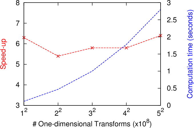
Table 4.2 makes it evident that the BDFT reduces the computation time by at least a factor of five over a range of (plausible) domain sizes, as visualized in Figure 4.4. Table 4.2 also reveals that the performance of the FFT implementation strongly depends on the transform size (which is proportional to the coherence length), because the algorithms selected by the FFTW library perform best with transform sizes that are products of small prime numbers. The BDFT algorithm, on the other hand, is insensitive to the transform size and scales at a constant rate with size.
| Hardware | Intel Core 3110M; 8 GB (dual channel) |
| OS | Ubuntu 13.10 (64 bit) |
| Compiler | gcc 4.8.1 |
| flags | -O3 -fastmath -march=native |
| FFT library | FFTW 3.3 (SIMD enabled) |
| interface \ flags | dft_r2c_2d \ FFTW_MEASURE |
| Ldev [a.u.] | Lcoh [a.u.] | BDFT [s] | FFT [s] | Speed-up [1] |
| 100 | 100 | 0.12 | 0.75 | 6.3 |
| 200 | 100 | 0.47 | 2.53 | 5.4 |
| 300 | 99 | 0.96 | 10.66 | 11.1 |
| 300 | 100 | 1.00 | 5.77 | 5.8 |
| 300 | 101 | 1.04 | 61.25 | 55.9 |
| 400 | 100 | 1.78 | 10.27 | 5.8 |
| 500 | 100 | 2.80 | 17.84 | 6.4 |
It is concluded that the presented box discrete Fourier transform (BDFT) algorithm is an efficient approach to compute the WP in a 2D domain, with a significant reduction in computation time. The BDFT algorithm can easily be extended to three dimensions and makes self-consistent solutions of the Wigner equation more feasible.
The semi-discrete formulation of the WTE (2.35) and the WP (4.1) rely on a finite coherence length to be chosen. The second important contribution made surrounding the WP concerns an analysis of the physical interpretation attributed to a chosen coherence length and its computational implications.
The Wigner theory is formulated for a coherence length approaching infinity. However, in a device, with dimensions Ldev, there does not exist coherence between any
two contacts, which limits the maximum coherence length to the dimensions of the device (separation of the contacts), i.e L = Ldev. Furthermore, in practical
computations the coherence length also cannot be taken to be infinite. When calculating (4.1) at any point other than the centre of the device, i.e. V W  ,
however, the boundaries of the device are exceeded and therefore the potential is unknown. Two different approaches to treat this situation are discussed in the
following.
,
however, the boundaries of the device are exceeded and therefore the potential is unknown. Two different approaches to treat this situation are discussed in the
following.
i) Regard any point outside the device to be in a contact region, which is assumed to maintain equilibrium conditions, and extend the potential value at the boundary as a constant or to ii) assume no coherence exists between the device and the contact region outside and progressively reduce the coherence length as the boundary is approached. Figure 4.5 reveals that the difference between these two approaches is significant. Approach ii) implies a decreasing value of Δk as the boundary is approached. To efficiently interpolate the values onto the fixed, finer, momentum grid, the potential difference in (4.1) is zero-padded at the front and the back. A further consideration when using approach ii) is that a shrinking coherence length implies that the portion of the potential profile considered for calculating the WP gradually reduces as the boundary is approached, up to the point, where the WP is no longer predominantly determined by the potential profile, but rather the length/width of the ’coherence box’ – a rectangular window with undesirable numerical effects, as will be discussed in the following section.
The coherence length is often associated with the distance over which quantum information, in the form of an electron state, is conveyed. Due to inelastic phonon scattering the electron state is changed and this information is lost. Based on this argument, an increase in the scattering rate suggests a decrease in the coherence length. However, the coherence length is often wrongly considered to be equivalent to the inelastic mean free path, as pointed out in, in two orthogonal dimensions, [134].
Further insight into the meaning of the coherence length can be gained from the scaling theorem – an analysis of a dimensionless, scaled version of the WBE, which considers the scales of the involved physical quantities: electron energy, electrostatic potential, phonon energy and electron-phonon coupling [49]. The analysis reveals that an increase of the electron-phonon coupling effectively reduces the distance over which the WP is ’felt’. Therefore, decoherence effects can be modelled through the choice of L itself, e.g. [135] considers an exponential damping of the WP, which essentially reduces L to model decoherence. Choosing a shorter coherence length can considerably reduce the computational burden of the simulation and is also justified, if the modelled decoherence processes reduce the effective coherence length sufficiently.
The physical considerations made to choose the coherence do not (significantly) depend on orientation. For computational convenience an isotropic coherence length is chosen such that |L| = L.
It is desirable to choose the coherence length as short as possible to limit the computational load of calculating the WP, which can be substantial in
multi-dimensional simulations. However, the coherence length also determines the momentum resolution, Δk =  , therefore, L must be chosen sufficiently large to be
able to differentiate the spectral content of different potential profiles. However, the attainable momentum resolution is limited by the dimensions of the device as
pointed out in the previous section.
, therefore, L must be chosen sufficiently large to be
able to differentiate the spectral content of different potential profiles. However, the attainable momentum resolution is limited by the dimensions of the device as
pointed out in the previous section.
Figure 4.6 shows different analytical potential profiles of the form
which suggest a sinusoidal potential variation, with a spatial frequency ω, superimposed on a potential bias (V 0 + mx).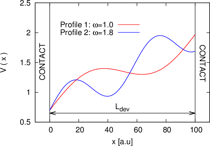
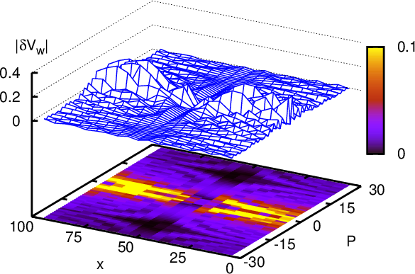
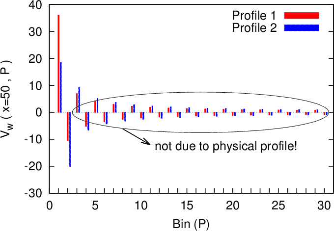
Since ω can be chosen, the values of the momentum index p (bins) of a 1D version of (4.4), which should be non-zero are known. If ω is chosen (ω = 1.0,1.8; cf. Figure 4.6) such that only the bins 1 and 2 of the corresponding WPs (at a fixed position) should be non-zero, Figure 4.7 reveals that this is not the case – there appear non-zero values at much higher-valued bins. These values at higher bins are not attributable to the physical profile, but are due to adverse effects, often termed ’spectral leakage’, inherent, when calculating a DFT of a non-periodic ’function’ over a finite length [136]. This situation is further exacerbated by the biasing condition which introduces a big discontinuity, because, when calculating the DFT, the potential profile is implicitly assumed to repeat periodically.
The preceding section has demonstrated situations where the components of the WP appear at values which cannot be attributed to a physical profile. Since the WP is normalized to represent a probability distribution for the generation of particles (see Section 3.7.5), the accumulated probability of the higher-valued bins (Figure 4.7) becomes significant and causes the generation of particles with very high momenta. The generation of these particles leads to a dramatic non-physical behaviour in the simulation. This section presents an approach that avoids this problem and represents an important step forward in attaining physically accurate simulation results with the WMC method. The results are based on [137] and are elaborated upon in the following.
To suppress the generation of particles which are not physically sound, a Tukey window function [138] is applied to taper the potential profile at the boundaries towards zero (or to the average value between the two boundary values), which yields a probability distribution that corresponds much better to the physical profiles. The smoothing mitigates the discontinuities introduced by the periodic repetition of the potential profile, which is implied when calculating a DFT.
Amongst the plethora of available window functions [136] – also known as tapering functions – the Tukey window (with α = 0.2; cf. Figure 4.8) was chosen with the physical motivation that it does not alter the physical profile inside the device noticeably. The Tukey window gives a coefficient with which sample n is multiplied and defined as
![(| 1[ ( (--2n--) )] α(N--1)
|{ 2 1+ cos π α(N-1) - 1 if 0 ≤ n < 2 ( )
w (n) = 1 if α(N2-1)≤ n < (N - 1) 1- α2- (4.8)
||( 1[ ( (--2n--) 2- )] ( α)
2 1+ cos π α(N-1) - α + 1 if (N - 1) 1- 2 ≤ n ≤ (N - 1)](html_diss_c267x.png)
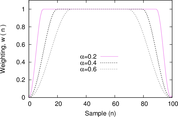
Figure 4.9 shows that by applying the Tukey window the (non-physical) higher bin values are suppressed, while the actual spectral components of the profile, at bins 1 and 2, remain pronounced. This results in a relative change of the probability distribution, which better reflects the physical situation in the device as illustrated by the following example.
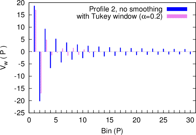
 , calculated at the centre of the device with and without the application of a smoothing
Tukey window (α = 0.2), using Profile 2 (blue) in Figure 4.6, and a coherence length of L = Ldev. The non-physical values revealed in Figure 4.7 are
suppressed by the application of the tapering window.
, calculated at the centre of the device with and without the application of a smoothing
Tukey window (α = 0.2), using Profile 2 (blue) in Figure 4.6, and a coherence length of L = Ldev. The non-physical values revealed in Figure 4.7 are
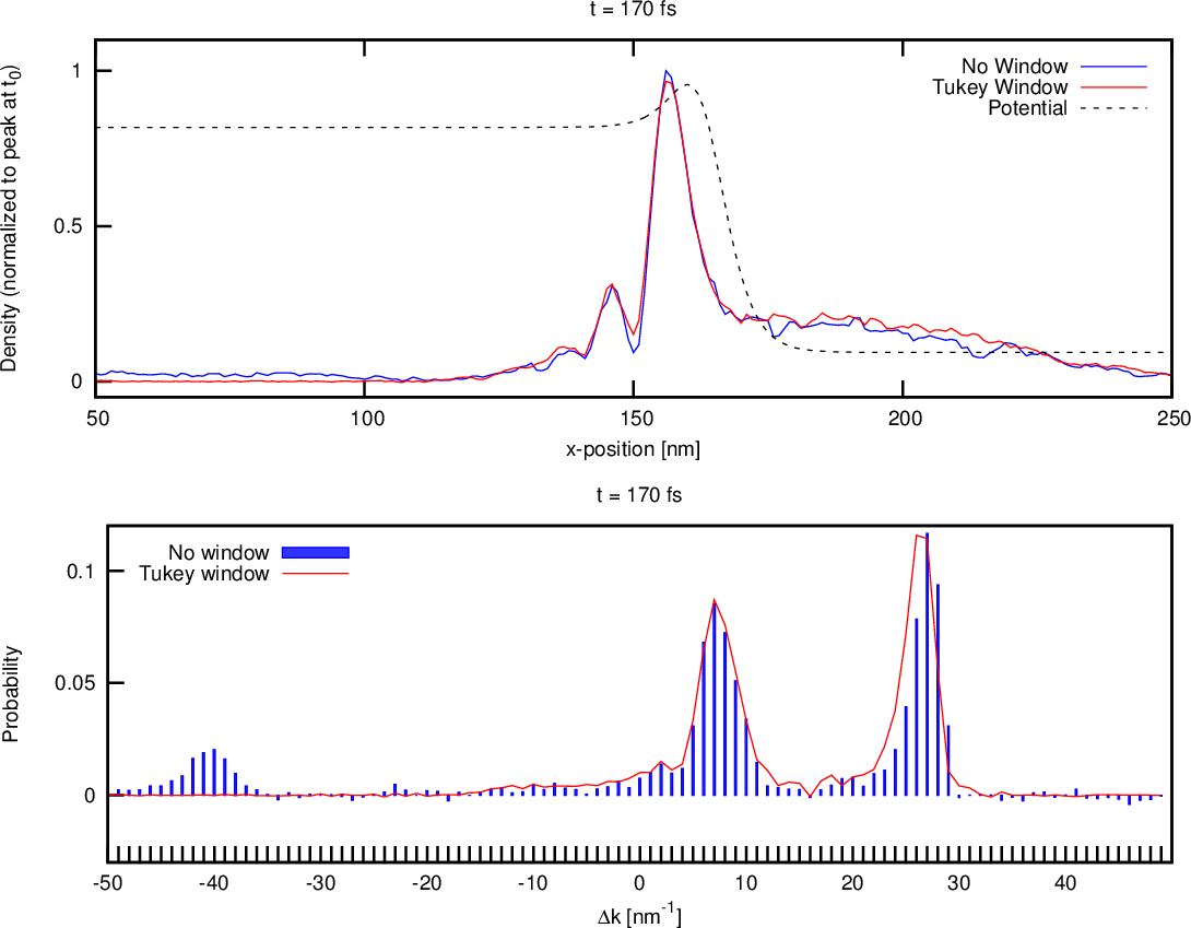
suppressed by the application of the tapering window.A practical example showing the importance of the tapering window is shown in Figure 4.10. A wavepacket travels, from the left, along a potential profile suggesting the channel (in transport direction) of a field-effect transistor (FET) with a k-distribution initially centred around 12Δk.
As the small potential barrier is approached a part of the wavepacket is slightly decelerated/reflected while the other part is accelerated by the big potential drop. An investigation of the (blue) k-distribution in Figure 4.10, however, reveals three peaks instead of the two suggested by physical considerations. The third (smallest) peak indicates a very strong reflection with a change in energy much larger than the potential difference between the left and the right contacts (boundaries). The latter is not physically grounded, but rather a consequence of the high-momenta particles being generated, if no tapering window is applied to treat the discontinuity introduced by the potential difference between the boundaries.
The application of a Tukey window function, which smooths the potential towards zero at the limits of the region of coherence, clearly remedies this problem (shown in red in Figure 4.10) and also avoids negative ’probabilities’ appearing in the k-distribution, leading to physically consistent results.


 , for the profiles in Figure