 (b)
(b)
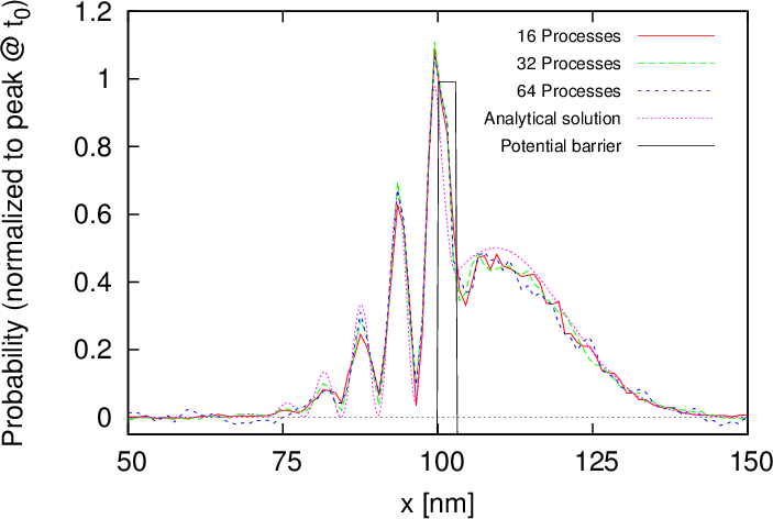
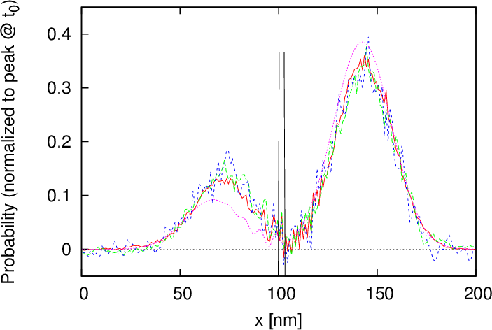
Figure 5.3: Comparison of the density of a wavepacket impinging on a 0.1eV, 3nm wide potential barrier for different numbers of MPI processes and an
analytical solution after (a) 85fs and (b) 125fs.
This section presents results obtained by the parallel algorithm introduced in the preceding section. First the parallelized algorithm is validated, whereafter its performance is evaluated with physical representative examples. The most important results obtained in [148] and [150], for 1D and 2D cases, are summarized here.
The spatial-decomposition approach must be validated to ensure that it yields the same results as the serial algorithm, regardless of the number of processes used, and does not introduce some (obvious) systematic errors, when the domain is split up.
Figure 5.3 shows the solution of a validation example – similar to the one described in Section 4.4 – for 16, 32 and 64 processes and compares it to the analytical solution. The parameters for the wavepacket and simulation are given in Table 5.1. An exact correspondence between the simulated results (within the bounds of the stochastic noise) is evident, irrespective of the number of processes used. This ensures the validity of the spatial domain decomposition approach. The slight deviation from the analytical solution – unlike the solution in Section 4.4 – is attributed to the much lower spatial resolution, which effectively gives the potential barrier a trapezoidal shape.
| x0 [nm] | σ [nm] | Lcoh [nm] | k0 [nm-1] | Δx [nm] |
| 40 | 7 | 100 | 18Δk | 0.1 |
(b)
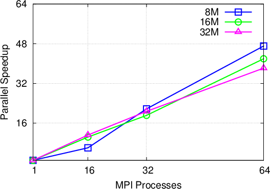
The parallel efficiency is evaluated based on the execution times of representative, physical examples in one and two dimensions. The simulations are first run with a single process, to acquire a baseline, and then repeated using 16, 32, 64 and 128 (2D case) processes. This procedure is repeated for different values for the maximum allowed ensemble size (8, 16 and 32 million particles). The maximum number of particles per process is scaled with the number of processes, e.g. a set maximum of 32 million particles for a simulation using 32 process, implies a maximum of 1 million particles per process. This scaling is necessary to allow a fair comparison. The execution time is recorded from the point where the master process starts the serial initialization and ends, when all process have completed the parallel time-loop (cf. Figure 5.2). All file output is disabled during the benchmarking.
The presented simulation results were obtained using (a part of) the VSC-3 supercomputer [151], which consists of 2020 nodes. Each node provides 16 cores (two 8-core Intel Xeon Ivy Bridge-EP E5-2650v2, 2.6GHz, Hyperthreading) and 64GB of system memory; the nodes are connected via an Intel QDR-80 dual-link high-speed InfiniBand fabric.
The parallel efficiency has been investigated in [148] at the hand of two examples presented in the following.
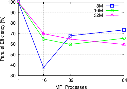
Single potential barrier: The first benchmark problem is the square potential barrier as used for validation purposes before. The parallel scaling is shown in Figure 5.4. A parallel efficiency of at least 60% is achieved for all cases. The only outlier is the case with a global particle maximum of 8 million particles, which shows a big jump in efficiency from 16 to 32 processes. This can be attributed to the annihilation process, which uses the maximum subensemble size per process as a criterion for performing an annihilation step, depending on the outcome of the growth prediction. For 16 processes each process is allowed a maximum of 500000 particles, whereas for 32 processes it is only 250000. This specific example shows an imbalanced concentration of particles in the form of the initial wavepacket; the larger subensemble maximum for 16 processes, allows for more growth before annihilation takes place and therefore can lead to a larger computational load overall.
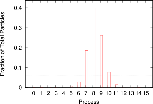
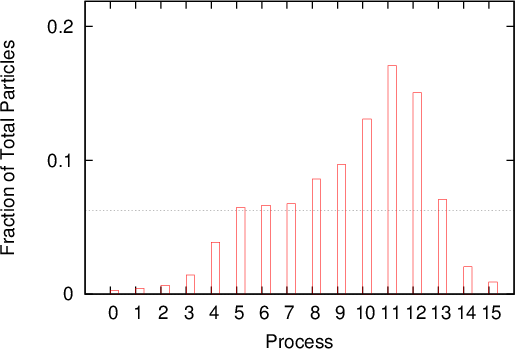
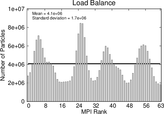
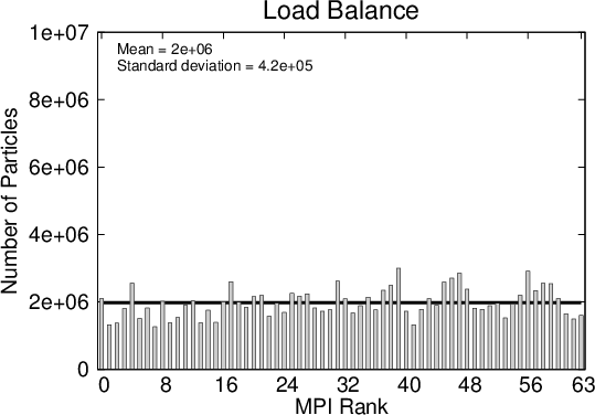
The absolute number of (numerical) particles within a subdomain serves as an indicator of the computational load a process experiences (the true load is also a function of the generation rate). Figure 5.5 shows the number of numerical particles at the same two time instances as in Figure 5.3.
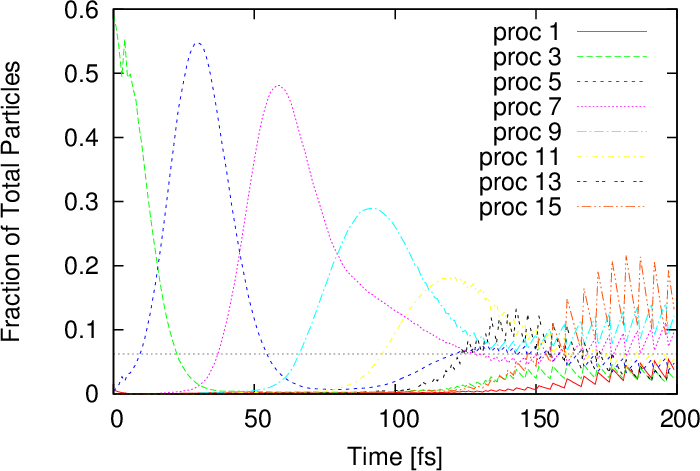
Figure 5.6 illustrates the time evolution of the number of particles on the processes. The evolution of the wavepacket travelling across the 200nm domain is clearly demonstrated by the initial imbalance of the workload on the processes. Initially, when the wavepacket is still narrow, the particles are passed on between the processes, but as the packet spreads the load distribution becomes more uniform. After approximately 150fs the distribution remains almost constant with some oscillations. The oscillations are due to the particle growth and annihilation taking place at regular intervals.
An important observations can be made from Figure 5.6: the ideal load per process is approached, when the evolution approaches a stationary regime. In light of this consideration, the next example starts with an initial condition which is already broadly spread out.
Double potential barrier: This example considers two wavepackets travelling towards each other in a domain with two potential barriers. The setup is the same as in the first example, apart from the location of the barriers and the initial position of the wavepackets, as stated in Table 5.2. A particle ensemble obtained after 80fs of evolution is used as an initial condition to start the simulation already with a good load-balancing between the processes.
| Parameter | Value | Unit |
| x01 | 40.0 | nm |
| k01 | 18Δk | nm-1 |
| x02 | 150.0 | nm |
| k02 | -18Δk | nm-1 |
| Barrier 1 width | 3.0 | nm |
| Barrier 1 left edge | 70 | nm |
| Barrier 1 height | 0.15 | eV |
| Barrier 2 width | 3.0 | nm |
| Barrier 2 left edge | 130 | nm |
| Barrier 2 height | 0.05 | eV |
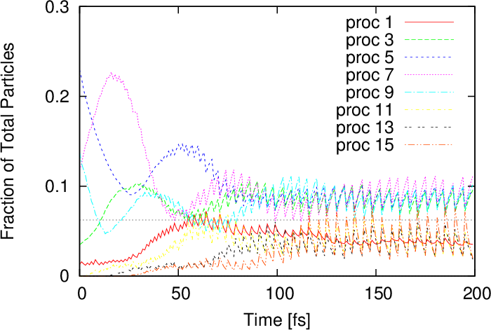
Figure 5.7 shows the parallel efficiency curves for the double barrier example, which is improved with respect to the single barrier case. This can be attributed to the improved load balancing amongst the processes from the initial condition. The evolution of the numerical particle distributions in Figure 5.8 shows how the load amongst the processes spreads out faster than for the single barrier problem. These peculiarities make the spatial decomposition method the ideal candidate for simulations of the stationary state, an example of which is shown in Section 6.2.
It is important at this point to underline the actual benefits of utilizing the presented parallelization approach in day to day research: the single barrier example, running on 64 processes with 60% efficiency, translates into a speed-up of around 40 times. In terms of execution time, the serial runtime of around 47 minutes was reduced to just 70 seconds. In the same vein, a simulation problem (of sufficient complexity), which would normally require two days of computation can be completed in approximately one hour. This aspect opens up a new realm of simulation problems, which can be investigated using the Wigner formalism.
The impact of the decomposition approach, slab- versus block-decomposition has been investigated in [150]. The main results are summarized here.
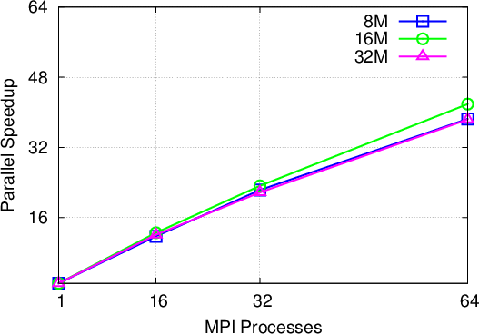
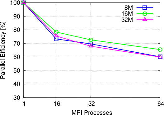
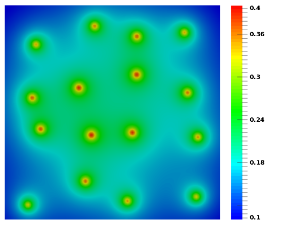
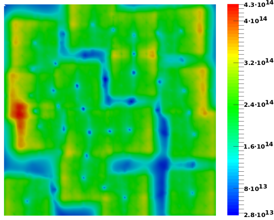
An example problem is considered with three minimum-uncertainty wave packages evolving over a 128nm × 128nm spatial domain. Sixteen non-identical acceptor dopants (positively charged) are spread across the domain, which yields the potential profile shown in Figure 5.9a and the corresponding particle generation rate γ depicted in Figure 5.9b. The particle generation rate is concentrated around each dopant within the region corresponding to the coherence length of 30nm. All boundaries are reflective, therefore, no particles leave the simulation domain. The maximum number of particles for the entire domain is limited to 64 ⋅ 107 particles; the local maximum for each process depends on the total number of processes used.
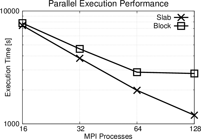
Figure 5.10 depicts the parallel execution performance for the slab and the block decomposition approach. The slab decomposition technique offers a significantly better parallel execution performance. The block decomposition method introduces a significant communication and requires additional logic, resulting in inferior performance relative to the slab decomposition approach. Especially for 128 MPI processes, the overhead triggers a stagnation of the scalability as the number of particles (work load) per process is too small relative to the additional communication overhead.
The memory consumption of the block-decomposition approach is slightly higher than for the slab-decomposition approach, due to the greater overhead for the communication and the related logic. However, this is negligible compared to memory requirements for sorting the particle ensemble and performing the annihilation algorithm.
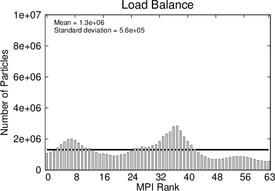
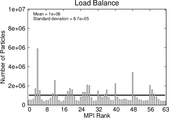
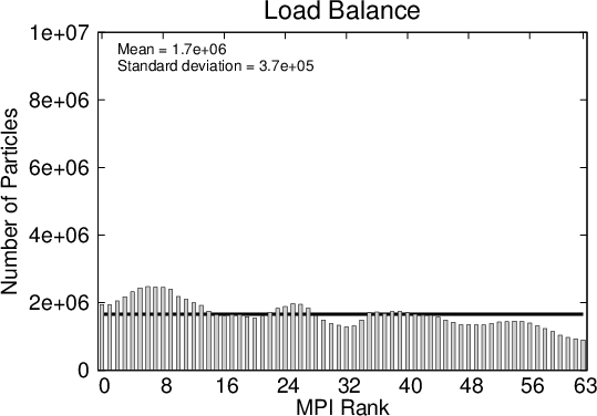
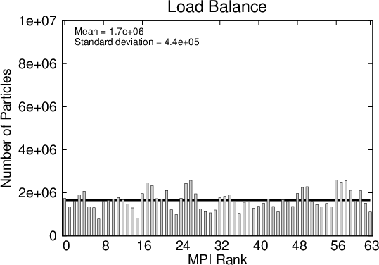
Although the load balance with the block decomposition appears to be better at the various time steps shown in Figure 5.11, the method’s performance is inferior to the approach using slab-decomposition. This is attributed to the additional communication and logic overhead incurred when using the block decomposition, which is between 1.5 to 4 times greater than in the case of slab-decomposition [150]. This result is particularly interesting, as the load balance does not appear to have a significant impact on the parallel scalability.
The annihilation procedure considerably reduces the number of particles (load) in a subdomain and is performed on an ’as-needed’ basis, which will differ for the various decomposition approaches. An average of the load over the entire simulation time paints the most realistic picture. Nonetheless, the snapshots of load balance at various times shown in Figure 5.11 already are useful, as they make clear that such differences exist.
This chapter has described the parallelization of the WEMC simulator using spatial domain decomposition, which has been deemed to be the best-suited for a large-scale parallelization in a distributed-memory system. The performance of the developed code has been evaluated and the slab-decomposition approach shows excellent parallel efficiency for two-dimensional simulations. This result has enabled the efficient use of high performance computing for two-dimensional Wigner Monte Carlo quantum simulations which facilitated the applications shown in Chapter 6.