6.1 Chemical Vapor Deposition

In [21], a simple model, which is able to describe low pressure CVD and PVD processes, was presented. It assumes ballistic particle transport at feature-scale and considers only a single particle species. Particles remain sticking on the surface according to a given sticking probability. Otherwise, the particles are reemitted from the surface, and their directions follow the Knudsen cosine law (2.18). For non-linear surface reactions, a dependence of the local sticking probability on the incident flux was derived (2.32), leading to a recursive problem.

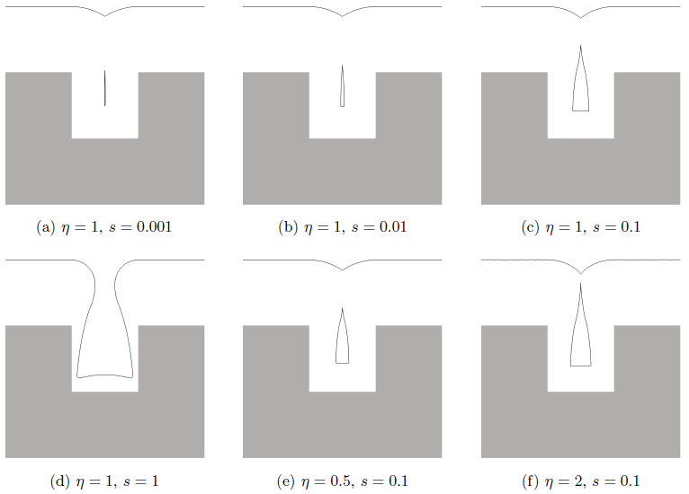
First, in order to compare the results and to verify the simulator, some two-dimensional low pressure CVD simulations, initially published in [21] are reproduced. The initial structure is a quadratic trench. The directional distribution of arriving particles is also assumed to obey a cosine distribution (2.5). The results for various sticking coefficients ${s}$ and reaction orders ${\eta }$ are shown in Figure 6.1. The value of ${s}$ corresponds, in the case of non-linear surface reaction ( ${\eta}\neq1$ ), to the sticking probability on a plane surface. The results are in good agreement with those given in [21].

Figure 6.1: Two-dimensional simulations of a deposition process for various sticking coefficients ${s}$ and reaction orders ${\eta }$ .

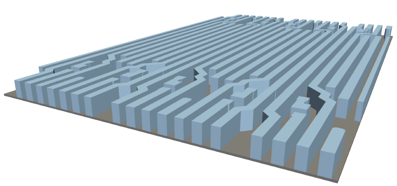
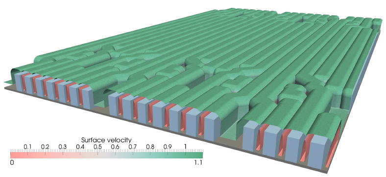
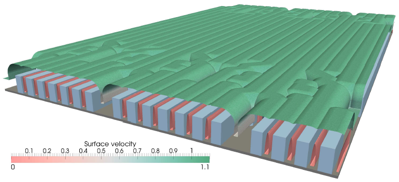
The well behaving scaling laws of all the numerical techniques allow the simulation of large three-dimensional structures. In order to demonstrate the capabilities of the simulator, a deposition process is simulated for a large initial structure as shown in Figure 6.2. Its lateral extensions are $1400\times 835$ grid spacings. The final profiles after deposition of a 15 and a 30 grid spacings thick layer are shown in Figure 6.3 and Figure 6.4, respectively. The deposition process was modeled using the parameters ${\eta}=1$ and ${s}=0.05$ .

Figure 6.2: The initial geometry was resolved on a grid with lateral extensions $1400\times 835$ .

Figure 6.3: The profile after deposition of a 15 grid spacings thick layer.

Figure 6.4: The profile after deposition of a 30 grid spacings thick layer.

For the simulation 1168 million particles are simulated at every time step in order to calculate the local deposition rates. Every time a particle hits the surface, a new particle is launched, as long as its new weight factor is larger than $0.001$ . The simulation was carried out in parallel on 24 cores of AMD Opteron 8435 processors ( $\SI {2.4}{\giga \hertz }$ ). The average calculation time for a time step is $\SI{10}{\minute}$ . In total, 600 time steps are necessary for the entire simulation, when using ${C_\text{CFL}}=0.1$ for the CFL criterion.