B. Ray-Isosurface Intersection

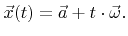
It is assumed that the surface is represented as the zero LS of function ${\Phi}({\vec{x}})$ and a ray with direction ${\vec{\omega}}$ passes through point ${\vec{a}}$

$${\vec{x}}(t)={\vec{a}}+t\cdot{\vec{\omega}}.$$ (B.1)

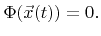
In order to find the intersection with the surface, the following equation must be solved

$${\Phi}({\vec{x}}(t))=0.$$ (B.2)

It is essential for ray tracing, that this equation can be solved with as few numerical operations as possible. Optimized algorithms are presented in the following, which are superior to those reported in the literature [69,74,88,119].

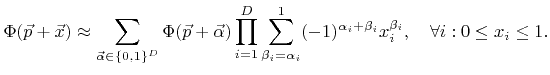
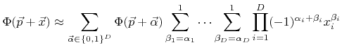
The LS function ${\Phi}$ is usually multi-linearly interpolated within a grid cell. The index vector of a grid cell is defined to be equal to the lower bound indices of all its corner grid points. For an arbitrary number of dimensions ${D}$ , the multi-linear interpolation formula within the grid cell with index vector ${\vec{p}}$ can be expressed as

$${\Phi}({\vec{p}}+{\vec{x}}) \approx \sum_{\vec{\alpha}\in\{0,1\}^... ...{1} (-1)^{\alpha_i+\beta_i} {x}_i^{\beta_i}, \quad \forall i : 0\leq{x}_i\leq1.$$ (B.3)

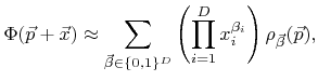
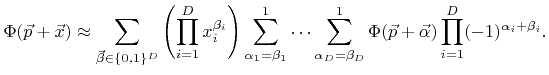
This expression can be expanded to a multi-variate polynomial

$${\Phi}({\vec{p}}+{\vec{x}}) \approx \sum_{\vec{\beta}\in\{0,1\}^{... ...\left( \prod_{i=1}^{{D}} {x}_i^{\beta_i} \right) \rho_{\vec{\beta}}({\vec{p}}),$$ (B.4)

where $\rho_{\vec{\beta}}({\vec{p}})$ are its coefficients. They can be obtained by rewriting (B.3) as

$${\Phi}({\vec{p}}+{\vec{x}}) \approx \sum_{\vec{\alpha}\in\{0,1\}^... ...a_{D}=\alpha_{D}}^{1} \prod_{i=1}^{{D}} (-1)^{\alpha_i+\beta_i} {x}_i^{\beta_i}$$ (B.5)

and further as

$${\Phi}({\vec{p}}+{\vec{x}}) \approx \sum_{\vec{\beta}\in\{0,1\}^{... ...}^{1} {\Phi}({\vec{p}}+\vec{\alpha}) \prod_{i=1}^{{D}} (-1)^{\alpha_i+\beta_i}.$$ (B.6)

Hence, the coefficients can be calculated as

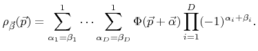$$\rho_{\vec{\beta}}({\vec{p}}) = \sum_{\alpha_1=\beta_1}^{1} \cdot... ...}^{1} {\Phi}({\vec{p}}+\vec{\alpha}) \prod_{i=1}^{{D}} (-1)^{\alpha_i+\beta_i}.$$ (B.7)

If the coefficients are calculated in a straightforward manner, $3^{D}-2^{D}$ additions or subtractions are needed [69,119]. However, the number of numerical operations can be reduced to $2^{{D}-1}{D}$ subtractions as demonstrated in Algorithm B.1. The algorithm is realized using template metaprogramming [2] which allows for the elimination of all recursive function calls at compile time. An array of size $2^{{D}}$ , which contains the LS values of all corner grid points in lexicographical order (with reversed significance), is passed to the static member function. After the function call the same array holds the coefficients $\rho_{\vec{\beta}}({\vec{p}})$ in lexicographical order (again with reversed significance) with respect to $\vec{\beta}$ .