3.2 Solving the Level Set Equation

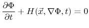
In this section numerical schemes for solving the LS equation are discussed. Since the LS equation belongs to the class of Hamilton-Jacobi equations

$$\frac{\partial{\Phi}}{\partial{t}}+{H}({\vec{x}}, \nabla{\Phi},{t})=0 \ {H}({\vec{x}}, \nabla{\Phi},{t})={V}({\vec{x}})\lVert\nabla{\Phi}\rVert$$ (3.4)

with ${H}$ denoting the Hamiltonian, many numerical schemes developed for the solution of Hamilton-Jacobi equations can also be applied to the LS equation.

Generally, the solution of a partial differential equation requires a discretization in time as well as in space. In case of the LS equation the simulation domain is usually discretized using regular grids which allow the application of simple finite difference schemes. In the following, ${\Delta x}$ denotes the grid spacing. Individual grid points are identified by an index vector ${\vec{p}}=\left({p}_1,\ldots,{p}_{D}\right)\in{\mathcal{G}}\subseteq\mathbb{Z}^{D}$ , where ${\mathcal{G}}$ denotes the set of index vectors of all grid points of the discretized simulation domain.

For regular grids the finite difference method is the most suitable method to solve the LS equation. As the name suggests, it approximates derivates by finite differences. The discretized version of (3.4) using the first-order forward Euler method [92] writes as

$${\Phi}^{({t}+\Delta{t})}({\vec{p}}) = {\Phi}^{({t})}({\vec{p}}) - \Delta{t}\cdot {\hat{H}}({\vec{p}},{\Phi}^{({t})},{V}({\vec{p}})).$$ (3.5)

Here ${\hat{H}}$ is an appropriate finite difference approximation to the Hamiltonian ${H}$ of the LS equation evaluated at grid point ${\vec{p}}$ . ${\hat{H}}$ depends on the discretized values of the LS function ${\Phi}^{({t})}$ at time ${t}$ and also on the current value of the velocity field ${V}({\vec{p}})$ at grid point ${\vec{p}}$ .

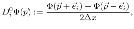
In the following discussion different approximations for the Hamiltonian are presented, which result in different time integration schemes. Since these approximations are based on finite differences, it is useful to introduce a notation for finite differences. The central difference operator is represented by ${D}^0_{i}$

$${D}^0_{i}{\Phi}({\vec{p}}):=\frac{{\Phi}({\vec{p}}+{\vec{e}}_i)-{\Phi}({\vec{p}}-{\vec{e}}_i)}{2{\Delta x}},$$ (3.6)

where ${\vec{e}}_i$ is the unit vector along the $i$ -th grid direction. Furthermore, the forward difference ${D}^+_{i}$ and the backward difference ${D}^-_{i}$ operator are defined as

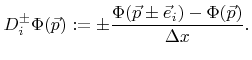$${D}^\pm_{i}{\Phi}({\vec{p}}):=\pm\frac{{\Phi}({\vec{p}}\pm{\vec{e}}_i)-{\Phi}({\vec{p}})}{{\Delta x}}.$$ (3.7)