3.4.2 The Sparse Field Method

A further development of the narrow band method is the sparse field method [135], which further reduces the computational effort by considering just a single layer of active grid points for time integration.

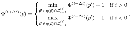
The method classifies all grid points ${\vec{p}}\in{\mathcal{G}}$ depending on their LS value as follows

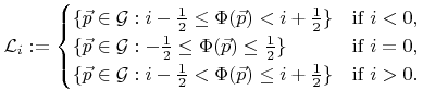$${\mathcal{L}}_i:= \begin{cases}\{{\vec{p}}\in{\mathcal{G}}: i-{\t... ...i}({\vec{p}})\leq {i+\textstyle\frac{1}{2}}\} & \text{if} \ i>0. \\ \end{cases}$$ (3.26)

The sparse field LS method assumes that from any two neighboring grid points with different signed LS values at least one belongs to ${\mathcal{L}}_0$

$$\forall {\vec{p}}\in{\mathcal{G}}, {\vec{p}}'\in{\eta}({\vec{p}})... ...ec{p}}')) \Rightarrow \{{\vec{p}},{\vec{p}}'\}\cap{\mathcal{L}}_0\neq\emptyset.$$ (3.27)

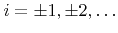
Here ${\eta}({\vec{p}})$ denotes the set of the closest neighbor grid points of ${\vec{p}}$ . In an infinite regular grid each grid point has $2{D}$ such neighbors, if ${D}$ is the number of dimensions. The signum function is assumed to be two-valued; $\funcsgn (0)$ can be either 1 or $\num{-1}$ . For numerical float data types the sign bit can be used to evaluate the sign. (3.27) is equivalent to the statement that the grid points with positive and negative signed LS values are separated by those belonging to ${\mathcal{L}}_0$ .

A further requirement of the sparse field LS method is that the layers ${\mathcal{L}}_i$ fulfill

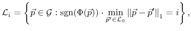$${\mathcal{L}}_{i}=\left\{{\vec{p}}\in {\mathcal{G}}:\funcsgn ({\P... ...{\vec{p}}'\in {\mathcal{L}}_{0}}{\lVert{\vec{p}}-{\vec{p}}'\rVert}_1=i\right\},$$ (3.28)

where $\lVert\cdot\rVert_1$ denotes the Manhattan norm. Once the grid points fulfill (3.26) to (3.28) the sparse field LS method can be applied. The method itself maintains these properties over time. A proper technique to initialize the LS values appropriately is described later in Section 4.1.1.

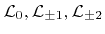
The idea of the sparse field method is now to consider only active grid points, namely those belonging to the most inner layer ${\mathcal{L}}_0$ , for time integration. However, the previously introduced numerical schemes also need the LS values of neighbor grid points, thus those of neighboring layers. For example, if second order derivatives are needed the LS values of grid points in layers ${\mathcal{L}}_{\pm 1}$ and ${\mathcal{L}}_{\pm 2}$ are required. After each time step, the LS values of non-active grid points must also be updated. Furthermore, the sets of grid points belonging to the individual layers may change and must be redetermined. The different sets of grid points ${\mathcal{L}}_i$ are originally represented as a list of pointers to the corresponding memory representations. The basic procedure of the sparse field method is presented in the following steps:

1. Update the LS values of all active grid points ${\vec{p}}\in{\mathcal{L}}_0^{({t})}$ in time using an appropriate finite difference scheme as described in the previous sections.
2. If there are any two neighboring grid points ${\vec{p}},{\vec{p}}'\in{\mathcal{L}}_0$ for which ${\Phi}({\vec{p}})<-\frac{1}{2}$ and ${\Phi}({\vec{p}}')>\frac{1}{2}$ the absolute LS values of both points are reduced to ${\Phi}({\vec{p}})=-\frac{1}{2}$ and ${\Phi}({\vec{p}}')=\frac{1}{2}$ , respectively.
3. In the order $i=\pm 1, \pm 2,\ldots$ the LS values of all grid points in the $i$ -th layer ${\vec{p}}\in {\mathcal{L}}_i^{({t})}$ are updated using

   $${\Phi}^{({t}+\Delta{t})}({\vec{p}})= \begin{cases}\displaystyle{\... ...}^{({t})}}{\Phi}^{({t}+\Delta{t})}({\vec{p}}')-1} & \text{if } i<0 \end{cases}.$$ (3.29)

   
   

4. Finally, the layers ${\mathcal{L}}_i^{({t}+\Delta{t})}$ for the next time step are determined using (3.26). Alternatively, due to the nature of the update scheme the determination of the layers using (3.28) is equivalent.

As previously mentioned, depending on the finite difference approximations used in the numerical update scheme a certain neighborhood around the active layer ${\mathcal{L}}_0$ is required. For example, if second order space schemes are used the availability of the LS values of all grid points in the layers ${\mathcal{L}}_0,{\mathcal{L}}_{\pm 1}, {\mathcal{L}}_{\pm 2}$ is sufficient. Consequently, the update rule (3.29) can be limited to grid points which are contained by these layers in the next time step.

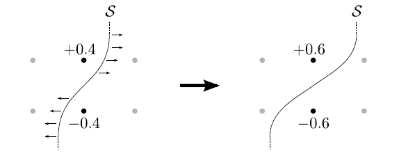
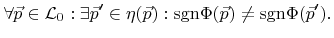
Item 2 does not exist in the original description of the sparse field method [135]. It has been proposed in [A18] to improve the robustness of the algorithm. If arbitrary velocity fields are allowed, cases may occur which contradict the assumption (3.27). As depicted in Figure 3.1 the update of the opposite signed LS values of two neighboring active grid points can lead to a pair of neighboring grid points, none of which belongs to ${\mathcal{L}}_0$ .

Figure 3.1: A problematic case which may occur and which needs special consideration. For the update of the neighboring pair of active grid points (black) with LS values $\pm 0.4$ opposite signed surface velocities (arrows) are used. This leads to a neighboring pair of non-active grid points with opposite signed LS values.

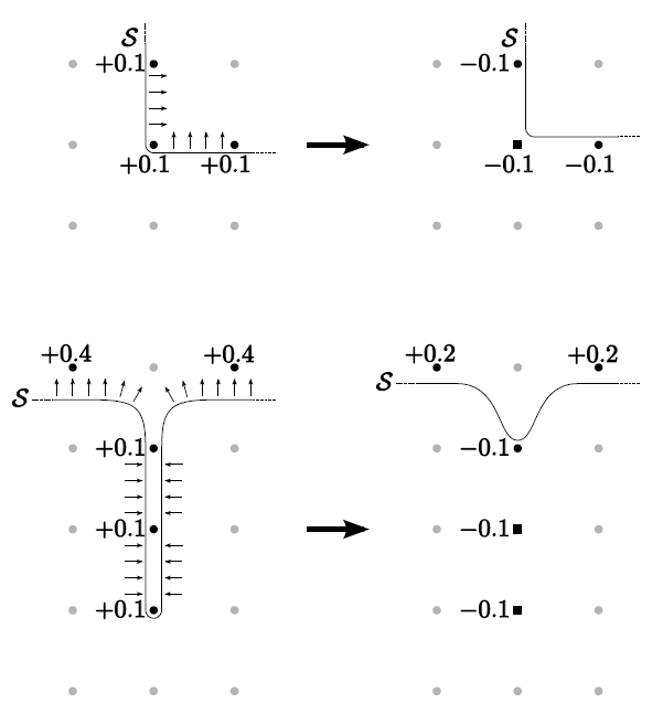
Another problem which may occur was already mentioned in the original paper [135]. The update scheme potentially leads to dense sets of active grid points, which do not have an opposite signed neighbor grid point. Figure 3.2 shows two examples, where so-called inefficient sets of active grid points are produced. They often appear in regions, where the surface converges, and do not necessarily need to be close to the surface afterwards, as illustrated by the second example. Hence, these points do not contribute to the description of the surface, and updating them is not necessary. The consideration of these non-relevant grid points makes the expansion of the surface velocity field more complicated and computationally more intensive. Even worse, dense sets of such points could be produced, essentially increasing the memory consumption and the calculation time during time integration. To avoid the accumulation of such active grid points a pruning procedure was proposed to keep ${\mathcal{L}}_0$ an efficient set of active grid points, so that each active grid point has an opposite signed neighbor point:

$$\forall {\vec{p}}\in {\mathcal{L}}_0: \exists {\vec{p}}'\in{\eta}({\vec{p}}):\funcsgn {\Phi}({\vec{p}})\neq\funcsgn {\Phi}({\vec{p}}').$$ (3.30)

The pruning procedure removes active grid points from ${\mathcal{L}}_0$ , which do not fulfill this criterion and finally updates all layers ${\mathcal{L}}_i$ and the corresponding LS values using (3.28) and (3.29), respectively. In Section 4.3 a robust algorithmic realization of the sparse field method including the pruning procedure will be presented.

Figure 3.2: Two examples, where the sparse field method produces inefficient sets of active (black) grid points. The surface ${\mathcal {S}}$ moves with a uniform positive surface velocity (arrows). After a time step some active grid points (squares) do not have a neighbor with opposite signed LS value.

For the sparse field method the CFL condition (3.15) can be written as

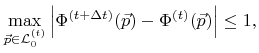$$\max_{{\vec{p}}\in {\mathcal{L}}_0^{({t})}} \left\vert {\Phi}^{({t}+\Delta {t})}({\vec{p}})-{\Phi}^{({t})}({\vec{p}}) \right\vert \leq 1,$$ (3.31)

which ensures that the surface advances at most one grid spacing per time step. For each step the time increment $\Delta{t}$ is chosen in such a way that

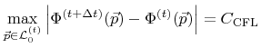$$\max_{{\vec{p}}\in {\mathcal{L}}_0^{({t})}}\left\vert{\Phi}^{({t}+\Delta {t})}({\vec{p}})-{\Phi}^{({t})}({\vec{p}})\right\vert = {C_\text{CFL}}$$ (3.32)

is fulfilled, where ${C_\text{CFL}}$ again denotes the predefined CFL number. A good choice for this positive constant is a value smaller than or equal to 0.5, which guarantees that only grid points of the active layer ${\mathcal{L}}_0^{({t})}$ change the sign of their LS value within a time step. This follows from the fact that the absolute LS values of grid points ${\vec{p}}\not\in{\mathcal{L}}_0^{({t})}$ are, according to (3.26), larger than 0.5 while the maximum change of the LS value is limited by ${C_\text{CFL}}$ , as stated in (3.32). The time step can be directly calculated by inserting (3.5) in (3.32)

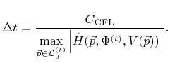$$\Delta{t} = \frac{{C_\text{CFL}}}{ {\displaystyle\max_{{\vec{p}}\... ...} \left\vert {\hat{H}}({\vec{p}},{\Phi}^{({t})},{V}({\vec{p}})) \right\vert } .$$ (3.33)

The sparse field method saves more computation time than the narrow band method for several reasons. First, only a minimal set of active grid points is involved in the time integration procedure. Furthermore, the time consuming surface velocity extension can be avoided. This extension is necessary for topography simulations, since the velocities are only defined on the surface and the LS method requires a velocity field [7]. Finally, the sparse field method does not require regular re-initializations, unlike the narrow band method [3]. The sparse field method was first applied in the field of topography simulation in [94].