4.6.1 Level Set Representation

For the following considerations the entire structure ${\mathcal{M}}$ is assumed to be composed of ${M}$ disjoint material regions ${\mathcal{M}}_1,{\mathcal{M}}_2,\ldots,{\mathcal{M}}_{M}$ satisfying (2.1). There are several possibilities to represent the different material regions by LS functions. One way is to describe each material region ${\mathcal{M}}_k$ by an enclosing LS function ${\Phi}_k$ [46]

$${\Phi}_{k}({\vec{x}})\leq0 \quad \Leftrightarrow \quad {\vec{x}}\in {\mathcal{M}}_k$$ (4.18)

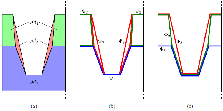
as shown in Figure 4.8b. However, using this representation, very thin layers with thicknesses smaller than one grid spacing cannot be properly resolved. However, some etching processes require the treatment of very thin passivation layers. If the passivation layer becomes thinner than the grid spacing, it can vanish abruptly, and the etching of the underlying material would start too early. This can lead to significant errors, especially for large etch rate ratios.

Figure 4.8: (a) A geometry consisting of 3 different materials, where ${\mathcal {M}}_1$ represents the substrate, ${\mathcal {M}}_2$ the mask, and ${\mathcal {M}}_3$ a passivation layer. (b) Description of the structure using 3 enclosing LSs. (c) Alternative representation where one LS describes the common surface and two others the interfaces between the different material regions.

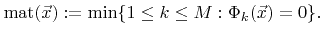
Instead, different material regions can be described by ${M}$ LS functions satisfying

$${\Phi}_{k}({\vec{x}})\leq0 \quad \Leftrightarrow \quad {\vec{x}}\in \bigcup_{i=1}^{k}{\mathcal{M}}_i.$$ (4.19)

Here ${\Phi}_{M}$ describes the surface of the entire structure ${\mathcal{M}}$ and the other LS functions correspond to interfaces as depicted in Figure 4.8c. This LS representation is often more convenient for topography simulation, because thin layers, such as the passivation layer ${\mathcal {M}}_3$ in Figure 4.8a, are described more accurately.

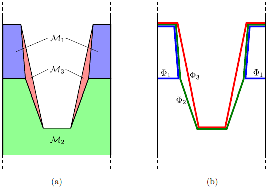
The LS configuration according to (4.19) depends on the numbering of the material regions. For comparison, a different LS representation, obtained through relabeling of the material regions is shown in Figure 4.9. The most suitable LS representation depends on the problem. If the mask is completely removed during the etch process, the configuration given in Figure 4.8c might be better. If underetching of the mask is expected, the LS representation shown in Figure 4.9b is favorable.

Figure 4.9: Renumbering of material regions (a) leads to a different LS representation (b).

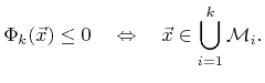
If the geometry is described using (4.19), the number of the material region which is on the surface can easily be determined using

$$\funcmat ({\vec{x}}):=\min\lbrace{1\leq k\leq {M}: {\Phi}_{k}({\vec{x}})=0}\rbrace.$$ (4.20)

$\funcmat$ is the surface material function which is defined for all surface points ${\vec{x}}\in{\mathcal{S}}$ .

For the following considerations all LS functions are assumed to fulfill

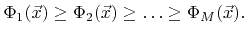$${\Phi}_1({\vec{x}})\geq{\Phi}_2({\vec{x}})\geq\ldots\geq{\Phi}_{M}({\vec{x}}).$$ (4.21)

This inequality is inherently satisfied, if the geometry is described by (4.19) and the LS functions are initialized as distance functions.

Some processes deposit new material layers on top of the structure. The described LS representation allows for easy additions of new material regions. It is sufficient to introduce a new LS function ${\Phi}_{{M}+1}$ , which satisfies 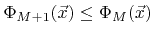${\Phi}_{{M}+1}({\vec{x}})\leq{\Phi}_{{M}}({\vec{x}})$ . In practice, to model the deposition of a new material, the new LS function is first initialized according to ${\Phi}_{{M}+1}({\vec{x}})={\Phi}_{{M}}({\vec{x}})$ . Then the LS equation is solved for this topmost LS function ${\Phi}_{{M}+1}$ , which represents the new surface. Stripping the top most material layer ${\mathcal{M}}_{M}$ is also very simple by deleting the top most LS function ${\Phi}_{{M}}({\vec{x}})$ .