


Next: 5.1.1 Algorithmic Complexity
Up: 5. Surface Rate Calculation
Previous: 5. Surface Rate Calculation
One way to calculate the surface rates is by direct integration. This requires
an appropriate discretization of the domain of the flux distribution function
 . Hence, the flux distribution at a certain surface point
  is approximated as a superposition of a finite number of appropriate basis functions
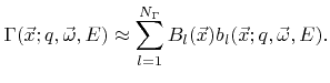 |
(5.1) |
 are the corresponding coefficients.
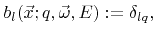
If the basis functions represent an orthonormal basis, thus
are the corresponding coefficients.
If the basis functions represent an orthonormal basis, thus
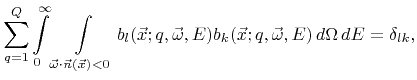 |
(5.2) |
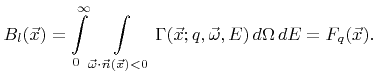
the coefficients
can be calculated using
 |
(5.3) |
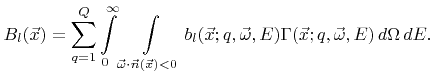
Insertion of the ballistic transport equation (2.14) yields
 |
(5.4) |
where  denotes the source term
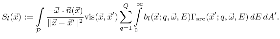 |
(5.5) |
Here,
 is the visibility function which returns 1 or 0, if the surface points
and
is the visibility function which returns 1 or 0, if the surface points
and
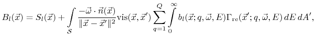
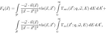
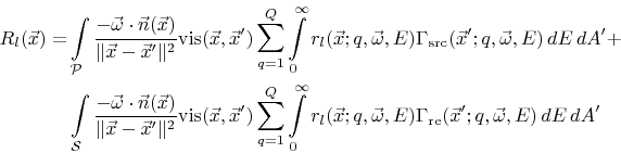
 are in line or sight or not, respectively. Utilizing expression (2.15) finally gives
 |
(5.6) |
with
 |
(5.7) |
To solve the surface integral equation (5.6) numerically, a discretization of the surface is needed. Triangle [68] or voxel elements [6] are conventionally used in three dimensions. If
 denotes the number of discretization elements of the surface, the number of unknowns is equal to
 . If
. If
 is large, thus if many basis functions are used to resolve the direction and energy dependence of the flux distribution, the number of variables, which must be kept in memory, is very large. This is especially a problem in three dimensions, where
is already very large by nature. Therefore, only a very small number of basis functions is commonly used in practice. Very often, only one basis function is used per particle type
is large, thus if many basis functions are used to resolve the direction and energy dependence of the flux distribution, the number of variables, which must be kept in memory, is very large. This is especially a problem in three dimensions, where
is already very large by nature. Therefore, only a very small number of basis functions is commonly used in practice. Very often, only one basis function is used per particle type
 |
(5.8) |
which reduces the number of unknowns to
 . As a consequence, the corresponding coefficients are equal to the respective total arriving flux of particles of species
 |
(5.9) |
The particle transport equation (2.14) simplifies to
 |
(5.10) |
and the reemitted flux distribution (2.15) can be written as
 |
(5.11) |
Here, the incident direction and the energy do not play a role in the reemitted flux distribution
 . The choice of the basis according to (5.8) assumes implicitly that the direction and the energy of reemitted particles is independent of the incident direction and energy. Therefore, effects such as specular-like reflexions of ions (see Section 2.2.3) cannot be accurately described, except for unidirectional and monoenergetic ion sources, for which the reemission probability function is the same for all incident ions.
Similarly, if the chosen basis is not able to reproduce the direction or the energy dependence of the arriving flux distribution  , the surface rates cannot be computed properly, given that they depend on the incident angle or energy. Hence, non-trivial surface rates, such as sputter rates, cannot be calculated correctly using the simple basis (5.8) and inserting (5.1) into (2.24). Only for unidirectional and monoenergetic particle incidence the sputter rates can be calculated correctly.
At least the contribution of primary particles, which come directly from the source plane
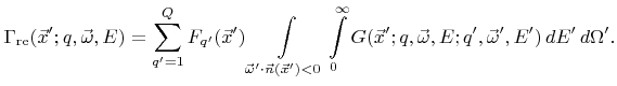
 , to the surface rates can be calculated correctly with reasonable effort using the simple basis (5.8). Once the coefficients
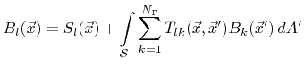
are calculated, the reemitted flux distribution can be approximated by inserting (5.1) into (2.15). Then the surface rates can be calculated using the formula
, to the surface rates can be calculated correctly with reasonable effort using the simple basis (5.8). Once the coefficients
are calculated, the reemitted flux distribution can be approximated by inserting (5.1) into (2.15). Then the surface rates can be calculated using the formula
 |
(5.12) |
which is obtained by combining (2.14) and (2.24).
Subsections
Next: 5.1.1 Algorithmic Complexity
Up: 5. Surface Rate Calculation
Previous: 5. Surface Rate Calculation
Otmar Ertl: Numerical Methods for Topography Simulation