


Next: 5.3.3 Direction Vector Calculation
Up: 5.3 Generation of Random
Previous: 5.3.1 Power Cosine Distribution
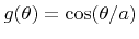
Next, the distribution introduced in (2.17) is considered, for which
 for all
![$ {\theta}\in\left[0,{\theta}_{\text{cone}}\right]$](img721.png) . Hence, all angles are within a cone with apex angle
. Hence, all angles are within a cone with apex angle
 . This is the reason for the name of the distribution used in this work.
  and
and
 are related by
 . To restrict the emission of particles to one hemisphere,
must satisfy
. To restrict the emission of particles to one hemisphere,
must satisfy
 , which is equivalent to
  . The probability density of the polar angle is given by
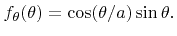 |
(5.40) |
The corresponding cumulative distribution function is
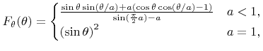 |
(5.41) |
Since it is not possible to calculate an explicit expression for the inverse function
 , which is useful for the inverse method, the rejection technique is chosen instead [25]. For the rejection method an instrumental distribution
 is necessary, which is an upper bound approximation of
 , and which leads to an invertable cumulative distribution function.
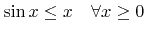
Using the inequalities
![$\displaystyle \cos{x} \leq 1-\left({\textstyle\frac{2}{\pi}}{x}\right)^2 \quad \forall {x}\in{\textstyle\left[-\frac{\pi}{2},\frac{\pi}{2}\right]}$](img732.png) |
(5.42) |
and
 |
(5.43) |
(see Inequality 1 and Inequality 2 in Appendix C) such an instrumental probability density function for (5.40) is given by
![$\displaystyle {f}'_{\theta}({\theta}) := \left(1-\frac{{\theta}^2}{{\theta}_{\t...
...theta}({\theta}) \quad \forall{\theta}\in\left[0,{\theta}_{\text{cone}}\right].$](img734.png) |
(5.44) |
The corresponding cumulative distribution function is
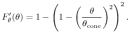 |
(5.45) |
According to the rejection method a random polar angle following
 can be generated by feeding the inverse of the instrumental cumulative distribution function
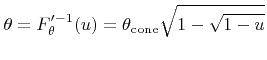 |
(5.46) |
with uniformly distributed random variates
![$ {u}\in\left[0,1\right]$](img738.png) and accepting
and accepting  , if
, if
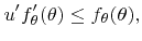 |
(5.47) |
where  denotes another uniformly distributed variate on
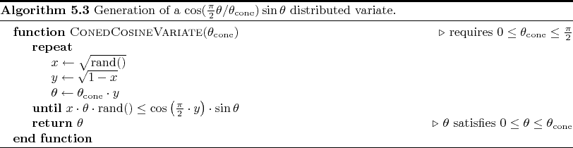
![$ \left[0,1\right]$](img715.png) . Algorithm 5.3 summarizes the entire procedure for determining random polar angles, which are distributed according to the coned cosine distribution.
. Algorithm 5.3 summarizes the entire procedure for determining random polar angles, which are distributed according to the coned cosine distribution.
The efficiency  of rejection sampling for this case, thus the fraction of successful attempts satisfying (5.47), is given by
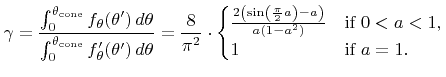 |
(5.48) |
The presented algorithm shows a very high efficiency, since
 holds for all
![$ {a}\in\left]0,1\right]$](img745.png) (see Inequality 3 in Appendix C), which corresponds to a success rate of approximately
(see Inequality 3 in Appendix C), which corresponds to a success rate of approximately
 in the worst case.
Next: 5.3.3 Direction Vector Calculation
Up: 5.3 Generation of Random
Previous: 5.3.1 Power Cosine Distribution
Otmar Ertl: Numerical Methods for Topography Simulation