Next: 5.3.4 Cosine Distribution
Up: 5.3 Generation of Random
Previous: 5.3.2 Coned Cosine Distribution
5.3.3 Direction Vector Calculation
Ray tracing usually requires a normalized direction vector. Therefore, once random polar and azimuthal angles with respect to the given unit vector  are determined, the direction vector
 can be obtained by
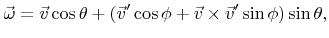 |
(5.49) |
where
 is a normal vector with respect to
, thus satisfying
is a normal vector with respect to
, thus satisfying
 . The rotational symmetry of the random direction distribution allows an arbitrary choice of
, which can be defined as follows
. The rotational symmetry of the random direction distribution allows an arbitrary choice of
, which can be defined as follows
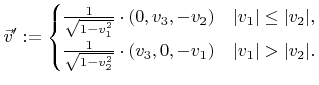 |
(5.50) |
The case differentiation avoids problematic cases, where
vanishes. In the following, only the first case is considered. The second case can be converted to the first case by exchanging the first two components of
,  and
and  , before calculating
. A final exchange of the corresponding components of
,
, before calculating
. A final exchange of the corresponding components of
,
 and
and
 , leads to the correct direction vector.
The condition
 together with
 implies
 and
and
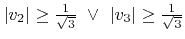 . Therefore,
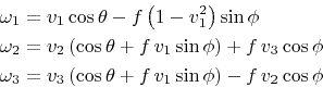
is always well-defined. Insertion into (5.49) gives
. Therefore,
is always well-defined. Insertion into (5.49) gives
with
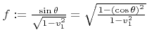 . Using the second notation of
  ,
can be calculated without knowledge of
,
can be calculated without knowledge of
 at the expense of one additional multiplication. Some distributions, such as the previously discussed power cosine distribution, enable the direct calculation of
 , avoiding the costly evaluation of trigonometric functions for the polar angle entirely (see the last note in Algorithm 5.2).
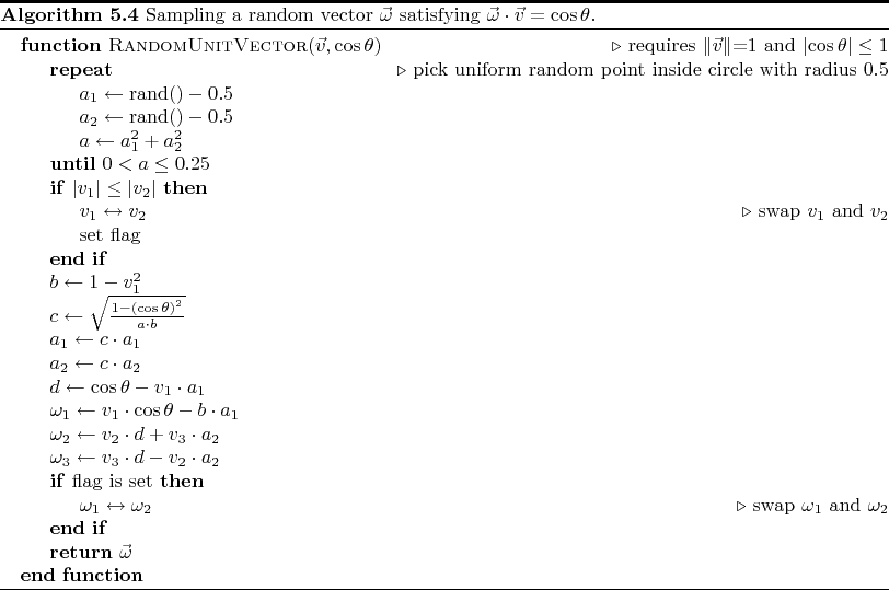
The evaluation of the other trigonometric functions in (5.51) can also be avoided. The point
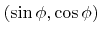 is uniformly distributed on the unit circle. An alternative way for picking a point on the unit circle is to randomly choose a point
  on a disk and to calculate the normalized vector
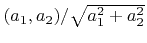 [25]. The radicand can be combined with that for the calculation of
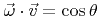
obviating the extra evaluation of the root. Algorithm 5.4 describes the determination of a random unit vector
around
with given polar angle
[25]. The radicand can be combined with that for the calculation of
obviating the extra evaluation of the root. Algorithm 5.4 describes the determination of a random unit vector
around
with given polar angle  , which is equivalent to
 .
.
Next: 5.3.4 Cosine Distribution
Up: 5.3 Generation of Random
Previous: 5.3.2 Coned Cosine Distribution
Otmar Ertl: Numerical Methods for Topography Simulation