Subsections
1.4.2 Surface Rate Calculation
When modeling topography evolution caused by traditional semiconductor processes with particle transport, the velocity field for
the LS equation must be found. This section discusses the particle transport to the surface and the surface reactions, which
are treated using a combination of fluxes and MC distributions.
The simulation domain is divided into the reactor-scale, feature-scale, and bulk regions, as
depicted in Figure 1.3. Particle transport must be treated differently when within the reactor-scale or
the feature-scale regions. The bulk region represents the silicon wafer.
Figure 1.3:
The simulation of particle transport, which is divided into the reactor-scale and feature-scale regions.
|
![\includegraphics[width=0.75\linewidth]{chapter_introduction/figures/transport.eps}](img70.png) |
The feature-scale region is separated from the reactor scale region by a flat plane
 depicted in Figure 1.3.
The particle transport is generally characterized by the mean free path
depicted in Figure 1.3.
The particle transport is generally characterized by the mean free path
 , which for an ideal gas is given by
 |
(8) |
where  is the Boltzmann constant,
  is the gas temperature,
  is the ambient pressure, and
  is the collision
diameter of a gas molecule. In the reactor-scale region, the mean free path is much smaller than the physical scale,
so the velocities of a neutral species can be assumed to follow the Maxwell-Boltzmann distribution, leading to a
cosine dependence of the flux distribution at
,
is the collision
diameter of a gas molecule. In the reactor-scale region, the mean free path is much smaller than the physical scale,
so the velocities of a neutral species can be assumed to follow the Maxwell-Boltzmann distribution, leading to a
cosine dependence of the flux distribution at
,

 |
(9) |
where  is the angle between the incident direction and the surface normal at the impact location.
 is the flux of neutral particles on
.
is the flux of neutral particles on
.
When ions are also used in transport, and not only neutral particles, their transport towards the wafer surface is modeled
by a plasma sheath potential. A narrower angle distribution is noted when compared to neutral particle transport, leading
to a power cosine distribution for charged particles
 |
(10) |
For large exponents  , this amounts to a normal distribution
 |
(11) |
The arrival flux of ions can then be expressed as
 |
(12) |
where
 is the normalized energy distribution. Plasmas which are based on RF
result in a more complex energy distribution which is solved using MC techniques. Most processes generate a
relatively even flux distribution
along
, excluding processes which include local particle
bombardments.
is the normalized energy distribution. Plasmas which are based on RF
result in a more complex energy distribution which is solved using MC techniques. Most processes generate a
relatively even flux distribution
along
, excluding processes which include local particle
bombardments.
The feature scale is encompassed by the plane
, the surface
 , and simulation domain boundaries
shown in Figure 1.3. The arriving flux
is known at
, while the re-emitted flux
distribution is given by
, and simulation domain boundaries
shown in Figure 1.3. The arriving flux
is known at
, while the re-emitted flux
distribution is given by
 for all points along the surface
. The summation of these two
fluxes determines the surface rates. The frequency of particle-particle interaction at the feature scale is
neglected for most processes [27].
for all points along the surface
. The summation of these two
fluxes determines the surface rates. The frequency of particle-particle interaction at the feature scale is
neglected for most processes [27].
The average particle velocity for an ideal gas particle is given by
 |
(13) |
where  is the gas molecular weight. The typical particle velocities are much higher than the surface rates, therefore
the surface rate can be seen as a constant and the time required for particles to reach the surface can be regarded as
relatively infinite with constant arrival at the substrate surface. The re-emitted arrival flux distribution must be known
in order to calculate the total flux at the surface
. The re-emitted flux distribution requires that
the reflected particle direction distribution also be known. This distribution can be generated by different cosine distributions
dependent on the particle type (ion, diffusive, or high-energy ion), while neutral particles are neglected. High energy
ions can sputter away pieces of the impacted surface, which deposit elsewhere. This is incorporated using a yield function,
which depends on the particle's incident energy
is the gas molecular weight. The typical particle velocities are much higher than the surface rates, therefore
the surface rate can be seen as a constant and the time required for particles to reach the surface can be regarded as
relatively infinite with constant arrival at the substrate surface. The re-emitted arrival flux distribution must be known
in order to calculate the total flux at the surface
. The re-emitted flux distribution requires that
the reflected particle direction distribution also be known. This distribution can be generated by different cosine distributions
dependent on the particle type (ion, diffusive, or high-energy ion), while neutral particles are neglected. High energy
ions can sputter away pieces of the impacted surface, which deposit elsewhere. This is incorporated using a yield function,
which depends on the particle's incident energy  , the threshold energy
  , and the incident angle
 |
(14) |
where  and
and  are fitting parameters.
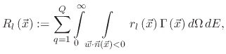
Therefore, the particle transport at the feature scale is described by
are fitting parameters.
Therefore, the particle transport at the feature scale is described by
 |
(15) |
where  is an infinitesimal surface element of
or
around
is an infinitesimal surface element of
or
around  .
.
This section summarizes the implementation of surface velocity calculations performed in the LS framework used for topography modeling from [50].
Once the particles have been transported to the surface, the deposition or etch rates can be found. These rates are needed in order to
find the velocity field
 which can be applied to the LS equation (1.3). The surface velocity can be
written as a function of all local arriving fluxes
which can be applied to the LS equation (1.3). The surface velocity can be
written as a function of all local arriving fluxes

 |
(16) |
In order to numerically represent the flux  , a discretization is performed. Introducing a series of functions
 with
with
 ,
can be mapped to a finite number of scalar values
,
can be mapped to a finite number of scalar values
 |
(17) |
where  is the number of process-relevant particle species,
  refers to a single particle species,
 is the number of surface rates, and
  represents the solid angle
between the particle direction and the surface normal at the point of impact.
The surface velocity is then found as a combination of the scalar values from (1.17)
represents the solid angle
between the particle direction and the surface normal at the point of impact.
The surface velocity is then found as a combination of the scalar values from (1.17)
 |
(18) |
When a particle of species  is accelerated to the surface its flux is determined by
 , where
 |
(19) |
This simplifies (1.17), since the information needed from the flux distribution for a certain particle type is mapped to a single value.
For high energy particles, the incident angle and energy are the values which are used to calculate the yield and the surface rate caused by
the particles. For an individual high energy particle of species , the total sputter rate determines its flux
 |
(20) |
The values of  represent the rates on the surface, whether they are referenced to a particle flux or a total sputter rate. Therefore,
they are interpreted as the surface rates, because
is a function of these rates
represent the rates on the surface, whether they are referenced to a particle flux or a total sputter rate. Therefore,
they are interpreted as the surface rates, because
is a function of these rates
 .
.
For systems with a linear surface reaction, the surface velocity is represented by the rates directly
 .
The surface velocity caused by a single species is modeled by
.
The surface velocity caused by a single species is modeled by
 |
(21) |
where  is the total incident flux,
  is the sticking probability of the reacting particles,
 is the mass deposited or removed
from the surface per particle, and
is the mass deposited or removed
from the surface per particle, and  is the bulk density
 .
.
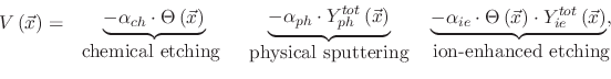
For non-linear surface reactions, where the sticking probability depends on the particle flux, the surface velocity is described using the
Langmuir adsorption model. The presence of multiple etchants, such as is the case for ion-enhanced etching, results in an etch rate
which is higher than that obtained by summing the individual contributions of the physical and chemical components. The etch rate
is composed of three contributions
 |
(22) |
where
 represents the coverage of the surface which is exposed to the adsorbed byproducts and is
expressed by
represents the coverage of the surface which is exposed to the adsorbed byproducts and is
expressed by
 |
(23) |
where the constants
 ,
,
 , and
, and
 are model-dependent parameters.
L. Filipovic: Topography Simulation of Novel Processing Techniques