Next: 2.3.4 Other One-Dimensional Oxide Up: 2.3 Linear Parabolic Description Previous: 2.3.2 Limitations of the
As previously described in Section 2.3.1, the Deal-Grove model can only describe oxidation growth for oxides
with thicknesses above 30nm. At the time when the Deal-Grove model was introduced (1965), the semiconductor industry
did not require such thin films. However, as the device sizes and geometries began to shrink, the limitations of the
Deal-Grove model became evident. It has been observed experimentally that the oxidation rate is much faster than predicted
by the Deal-Grove model at the initial stages of oxidation and for thin oxide growths [34].
Several researchers have suggested that the cause of the increased oxidation
rate are electrochemical effects such as field-enhanced oxidation, structural effects such as microchannels, stress effects
modifying oxidant diffusivity, and changes in oxygen solubility in the oxide with little success. Those that had more success
suggested the increased rate is due to parallel oxidation mechanisms such as silicon interstitials injected into the oxide, oxygen vacancies,
diffusion of atomic oxygen, surface oxygen exchange, and the effects of a finite non-stoichiometric transition region between
amorphous SiO![]() and Si [34].
and Si [34].
Massoud et al., in 1985 [143], [144] suggested an update to the Deal-Grove model for dry oxidation, which was to address the thin oxide growth regime. They provided an analytical model based on parallel oxidation mechanisms to fit experimental data with good success. The price for the improved model for thin oxides is an increased complexity of the model.
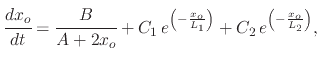
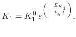
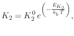
Massoud introduced additional terms to the oxidation rate equation (2.16) and changed the values of the linear and parabolic constants. The oxidation rate is given by
The values for the pre-exponential constants ![]() ,
,
![]() and the activation energies
and the activation energies ![]() ,
,
![]() for
different crystal orientations and temperatures are listed in Table 2.3. It should also be noted that the values
for
for
different crystal orientations and temperatures are listed in Table 2.3. It should also be noted that the values
for ![]() ,
,
![]() ,
, ![]() , and
, and
![]() change with temperature, which was not the case with the original Deal-Grove
model.
change with temperature, which was not the case with the original Deal-Grove
model.
| ||||||||||||||||||||||||||||||||||||
In (2.37), the second and third term on the right hand side are additional terms which represent the rate enhancement in
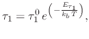
the thin regime. They are defined by pre-exponential constants ![]() and
and ![]() and characteristic lengths
and characteristic lengths ![]() and
and ![]() . The first
characteristic length
. The first
characteristic length ![]() is in the order of 1nm and is meant to deal with the rate increase in the first 5nm of oxide growth,
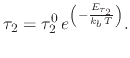
after which it vanishes. The second characteristic length
is in the order of 1nm and is meant to deal with the rate increase in the first 5nm of oxide growth,
after which it vanishes. The second characteristic length ![]() , with a value in the order of 7nm, is meant to decay until approximately
25nm, after which it no longer influences the oxidation rate and the rate becomes linear-parabolic once again.
, with a value in the order of 7nm, is meant to decay until approximately
25nm, after which it no longer influences the oxidation rate and the rate becomes linear-parabolic once again.
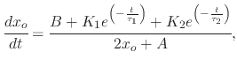
Another way to express (2.37) in terms which are easier to manipulate and mathematically solve is presented in [142]
The pre-exponential constants and activation energies of the above expressions (2.41)-(2.44)
are given in Table 2.4 for dry oxidation in a temperature range from 800-1000
![]() C.
C.
|
As already performed for the Deal-Grove expression in Section 2.3.1, inverting (2.40) gives a convenient expression for the oxide thickness as a function of oxidation time and vice-versa. Therefore, (2.40) is re-written as
Equation (2.46) can be solved in order to obtain an analytic expression for the oxide thickness as a function of oxidation time
The relationship (2.48) is meant to give a valid expression for the oxide thickness after an oxidation
time ![]() in a dry ambient from the native oxide thickness conditions. Figure 2.13 shows the difference between
the Deal-Grove model and the Massoud model for the initial stages of oxidation. It is evident that the Massoud model depicts
a faster initial oxidation rate.
in a dry ambient from the native oxide thickness conditions. Figure 2.13 shows the difference between
the Deal-Grove model and the Massoud model for the initial stages of oxidation. It is evident that the Massoud model depicts
a faster initial oxidation rate.
![\includegraphics[width=0.70\linewidth]{chapter_oxidation/figures/dg_massoud.eps}](img314.png) |
![$\displaystyle \left(2x_{o}+A\right)dx_{o}=\left[B+K_{1}\,e^{\left(-\frac{t}{\tau_{1}}\right)}+K_{2}\,e^{\left(-\frac{t}{\tau_{2}}\right)}\right]dt$](img307.png)
![$\displaystyle x_{o}^{2}+Ax_{o}=B\cdot t+M_{1}\left[1-e^{\left(-\frac{t}{\tau_{1}}\right)}\right]+M_{2}\left[1-e^{\left(-\frac{t}{\tau_{2}}\right)}\right]+M_{0},$](img308.png)
![$\displaystyle x_{o}=\sqrt{\left(\cfrac{A}{2}\right)^{2}+B\cdot t+M_{1}\left[1-e...
...+M_{2} \left[1-e^{\left(-\frac{t}{\tau_{2}}\right)}\right]+M_{0}}-\cfrac{A}{2}.$](img313.png)