Subsections
The simulator is implemented by first calculating the shape of the nanodot or nanowire
with the previously mentioned empirical equations which
depend on the oxidation time, applied voltage, ambient humidity, and nanowire orientation.
Afterwards, a given number of particles is distributed above the silicon surface,
their position following the pattern of the desired surface deformation. Finally, each particle
is accelerated towards the surface, causing it to collide with the wafer. Upon impact, the silicon
dioxide is advanced deeper into the silicon, while it simultaneously grows into the ambient. The result
is an oxide nanodot or nanowire having the desired height and width, depending on the processing variables
of voltage, time, humidity, and orientation. The method of imprinting a desired particle distribution
onto a wafer surface is represented graphically in Figure 3.19.
Figure 3.19:
Image representation of the MC method of ``imprinting'' a desired particle distribution onto the silicon
surface in order to generate an oxide growth. The particles are accelerated using ray tracing techniques within
the LS simulator environment.
|
![\includegraphics[width=\linewidth]{chapter_process_modeling/figures/AFM_distribution.eps}](img470.png) |
A flow chart summarizing the simulation steps is given
in Figure 3.20, which describes how the desired particle distribution is effectively imprinted
onto the LS surface using the MC method.
Figure 3.20:
Flow chart of the simulation process implementing the Monte Carlo method with ray tracing in a LS environment.
![\includegraphics[width=0.9\linewidth]{chapter_oxidation_modeling/figures/flowchart.eps}](img471.png) |
As seen from the previous discussion regarding the MC model for AFM oxidation from Figure 3.20,
a method to distribute particles according to a desired distribution is required.
Some literature approximate the final oxide dot topography with a Gaussian curvature [162], while some suggest a
Lorentzian profile [84].
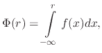
The quantile function of the one-dimensional Gaussian distribution, required for the generation
of a random particle position  , is
, is
 erf erf |
(123) |
Because of the error function, the quantile Gaussian function is not easily implementable with a random distribution
in the MC environment
and hence another model is desired. The model implemented in the simulator is based on the well known
Marsaglia polar method [139]. This method suggests a way to generate two
independent standard normal random variables. The first step is the generation of an evenly distributed
random location (r , r
, r ) within a circle of unity radius
 , where r and r are evenly
distributed random numbers
, where r and r are evenly
distributed random numbers  (-1, 1). The Gaussian distributed coordinates (x
 , y) can then be calculated
using the Marsaglia equations
, y) can then be calculated
using the Marsaglia equations
 |
(124) |
A sample Gaussian distributed nanodot is shown in Figure 3.21.
Figure 3.21:
Nanodot generated using Gaussian particle distribution. The vertical dimension has been scaled by 20 for better visualization.
(a) NCM nanodot generated using a Gaussian distribution of particles and (b) Diagonal cross-section of the nanodot from Figure 6.13a
|
![\includegraphics[width=0.481\linewidth]{chapter_process_modeling/figures/gaussian_dot.eps}](img481.png) |
![\includegraphics[width=0.481\linewidth]{chapter_process_modeling/figures/gaussian_dot2.eps}](img482.png) |
| (a) NCM Gaussian nanodot |
(b) Cross-section. |
|
The Gaussian distribution is well known; however from Figure 3.22, it is suggested that a Lorentzian distribution is a better fit to the
final shape of the desired nanostructure [84].
Figure 3.22:
(a) Comparison between the Gaussian distribution and the surface charge density and (b) comparison between the
Lorentzian distribution and the surface charge density.
|
![\includegraphics[width=0.481\linewidth]{chapter_process_modeling/figures/gauss_charge.eps}](img483.png) |
![\includegraphics[width=0.481\linewidth]{chapter_process_modeling/figures/lorentz_charge.eps}](img484.png) |
| (a) Gaussian distribution. |
(b) Lorentzian distribution. |
|
The implementation of the Gaussian distribution was performed successfully, while a similar
approach to the Lorentzian distribution was attempted without much success. Therefore,
in order to generate particles according to a Lorentzian distribution, a novel
technique for a particle distribution which follows the Lorentzian equation is developed.
The technique results in equations similar to the Marsaglia-Polar equations from (3.53).
- One-Dimensional Distribution
The normalized Probability Density Function (PDF) of the Lorentzian distribution is given by:
 |
(125) |
The Cumulative Probability Density (CPD) is found by integrating the PDF to obtain
 |
(126) |
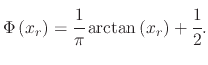
The quantile function of the Lorentzian distribution, required for particle generation, is
the inverse CPD
![$\displaystyle x_r=\Phi^{-1}\left(\xi\right)\equiv\tan\left[\pi\left(\xi-\cfrac{1}{2}\right)\right],$](img488.png) |
(127) |
where
 is a uniformly distributed random number. Therefore, using (3.56), a random
particle can be generated to follow the Lorenzian distribution by first generating an evenly distributed value for
is a uniformly distributed random number. Therefore, using (3.56), a random
particle can be generated to follow the Lorenzian distribution by first generating an evenly distributed value for  .
.
- Two-Dimensional Distribution
The same analysis shown for the one-dimensional Lorentzian distribution must be performed in order
to generate a two-dimensional Lorentzian quantile function. The two-dimensional Lorenzian distribution is required
when a three-dimensional nanodot needs to be simulated.
The PDF of the two-dimensional Lorentzian distribution can be represented as
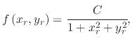 |
(128) |
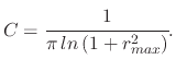
where  is the normalization constant. Using polar coordinates, where
 and
and
 , it can easily be shown that
the PDF cannot be normalized in the entire real space
, it can easily be shown that
the PDF cannot be normalized in the entire real space  . We therefore must
normalize the equation to a desired maximum radius
. We therefore must
normalize the equation to a desired maximum radius  .
.
 |
(129) |
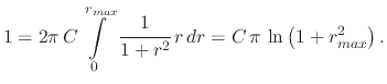
The normalization constant follows from the CPD, normalized to
 |
(130) |
The CPD for the two-dimensional distribution, normalized to can then be written as
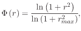 |
(131) |
where
 is treated as a -dependent
constant
is treated as a -dependent
constant  . By inverting the CPD and solving for
  the two-dimensional Lorentzian
quantile function is found, which is required for particle generation
the two-dimensional Lorentzian
quantile function is found, which is required for particle generation
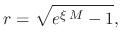 |
(132) |
where
is a uniformly distributed random number. Using (3.61), a random
particle location can be generated in two-dimensional space to follow the Lorenzian distribution.
The generated location is a radial distance from the center of the distribution.
An evenly distributed angle  between 0 and 2
 is generated and the final
particle position is given by
is generated and the final
particle position is given by
 .
It can be observed that the choice of affects the height of the Lorentzian
distribution, thereby affecting the height of the desired nanodot. Therefore,
an additional contribution, dependent on , is needed in the equation for the
height generated by each particle. This contribution is
.
It can be observed that the choice of affects the height of the Lorentzian
distribution, thereby affecting the height of the desired nanodot. Therefore,
an additional contribution, dependent on , is needed in the equation for the
height generated by each particle. This contribution is
 |
(133) |
The resulting nanodot cross section, shown in Figure 3.23 matches
the ideal one-dimensional Lorentzian distribution. This method allows the
generation of nanodots, such as the one shown in Figure 3.24,
which follow a Lorentzian distribution, as desired for the AFM oxidation simulator.
Figure 3.23:
Cross-sectional nanodot height generated using a Lorentzian distribution.
|
![\includegraphics[width=0.6\linewidth]{chapter_process_modeling/figures/Attempt2_2.eps}](img505.png) |
Figure 3.24:
The vertical dimension has been scaled by 20 for better visualization.
(a) NCM nanodot generated using a Lorentzian distribution of particles and (b) Diagonal
cross-section of the nanodot
from Figure 3.24a.
|
![\includegraphics[width=0.481\linewidth]{chapter_process_modeling/figures/lorentzian_dot.eps}](img506.png) |
![\includegraphics[width=0.481\linewidth]{chapter_process_modeling/figures/lorentzian_dot2.eps}](img507.png) |
| (a) NCM Lorentzian nanodot. |
(b) Cross-section. |
|
The expression for the quantile function in (3.61) suggests a potential
connection to the Marsaglia polar method. A Lorentzian distribution can be generated
using a similar procedure. The first step is, once again, the generation of an evenly distributed random
location in two dimensions
 within a circle with radius
.
The Lorentzian distributed coordinates
within a circle with radius
.
The Lorentzian distributed coordinates
 can then be expressed as:
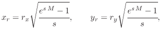 |
(134) |
where
 .
.
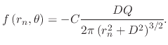
SCD charge density on the
silicon wafer is advantageous since a nanodot can then be generated which directly follows the applied electric field, a function
of the applied voltage at the AFM needle.
When performing nanodot oxidation simulations using an AFM for a two-dimensional model, a one-dimensional
particle distribution is required. The equation (3.37), for a SCD distribution of
a hemispherical needle tip can be re-written in a one-dimensional form:
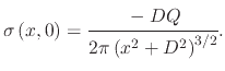 |
(135) |
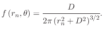
(3.64) can then be used to generate a one-dimensional PDF
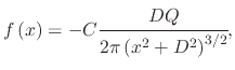 |
(136) |
where is the normalization constant. is found by integrating
 over the entire
simulation domain and equating it to unity:
over the entire
simulation domain and equating it to unity:
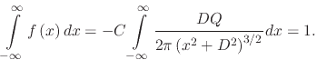 |
(137) |
By solving (3.66), the normalization constant is found
 |
(138) |
which is then substituted into (3.65) to form the normalized PDF for a one-dimensional SCD distribution
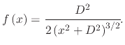 |
(139) |
The next step is finding the CPD function, derived by integrating the normalized PDF,
 |
(140) |
where is the SCD distributed
radius. Because of the symmetry of the SCD distribution on either side of the charged
particle  , generating a CPD distributed radius becomes easier, when
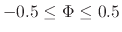 .
Therefore, we set
.
Therefore, we set
 |
(141) |
leading to
 |
(142) |
Setting  equal to an evenly distributed random number
 and inverting
(3.71) allows us to obtain the SCD quantile function required for
particle generation:
and inverting
(3.71) allows us to obtain the SCD quantile function required for
particle generation:
 |
(143) |
Therefore, in order to generate particles obeying the SCD distribution along the silicon
wafer surface, each particle must be generated using (3.72), where is an evenly
distributed random number,
.
When working with a three-dimensional model for AFM oxidation of nanodots, a two-dimensional
particle distribution is required. The analysis is similar to the one-dimensional
model presented in the previous section. The derivation of the quantile
function is performed using polar coordinates for simplicity and for easier generation of a
final radial distribution of particles. For polar coordinates
 it is important to note
that
it is important to note
that
 , and
, and
 . This was also discussed when deriving the Lorentzian distribution.
The two-dimensional PDF, in polar coordinates, derived from (3.37) is
. This was also discussed when deriving the Lorentzian distribution.
The two-dimensional PDF, in polar coordinates, derived from (3.37) is
 |
(144) |
The normalization constant is once again found by integrating the PDF over the entire simulation range and equating it to
one:
 |
(145) |
then the normalized two-dimensional PDF in polar coordinates becomes
 |
(146) |
The CPD is found by integrating the normalized PDF over the simulation area. The angular component results in a value of 2, while
the radial component is found by first finding the radius-dependent CPD
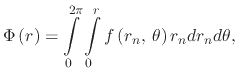 |
(147) |
which equates to
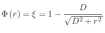 |
(148) |
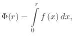
The quantile function for the two-dimensional SCD distribution is found by inverting the CPD
function to obtain
 |
(149) |
where is an evenly distributed random number,
 . The angular component of the distribution is obtained in the same
manner as the radial component for the Lorentzian distribution. An evenly distributed angle
. The angular component of the distribution is obtained in the same
manner as the radial component for the Lorentzian distribution. An evenly distributed angle  between 0 and
  is found and the
final Cartesian location for each particle is given by
is found and the
final Cartesian location for each particle is given by
 .
The normalized cross-section of a nanodot generated using this distribution is compared to
the normalized SCD from (3.64) in Figure 3.25.
.
The normalized cross-section of a nanodot generated using this distribution is compared to
the normalized SCD from (3.64) in Figure 3.25.
Figure 3.25:
Normalized effective nanodot cross section height and the normalized SCD function.
|
![\includegraphics[width=0.65\linewidth]{chapter_process_modeling/figures/cross-sect.eps}](img538.png) |
As previously mentioned, a rough needle tip must be modeled using a ring of charges at a given height above the silicon
surface. The SCD distribution is found using the method of image charges and summing the effects of each individual
charge which makes up the charged ring, resulting in the SCD distribution shown in (3.38).
The SCD in (3.38) does not allow for a straight-forward derivation
of a random distribution, such as the one shown in (3.72) and (3.78).
Therefore, the MC rejection technique, or the accept-reject algorithm must be applied, whereby a test point is generated on the entire
simulation domain using an even distribution,
 . An additional
evenly distributed number between zero and
. An additional
evenly distributed number between zero and
 from (3.39) is generated and, if this number is
below
from (3.39) is generated and, if this number is
below
 , a particle is generated at
 .
Otherwise, the location
is ignored and a new test point is generated.
This procedure is repeated until a sufficient number of particles is kept in order to generate
a nanodot topography.
.
Otherwise, the location
is ignored and a new test point is generated.
This procedure is repeated until a sufficient number of particles is kept in order to generate
a nanodot topography.
Figure 3.26:
The effective diagonal cross-section height of a nanodot when using a rough AFM needle tip versus a hemispherical AFM needle tip.
|
![\includegraphics[width=\linewidth]{chapter_process_modeling/figures/Hemispherical.eps}](img543.png) |
It is evident that a blunt needle tip
will result in a blunt nanodot formation with a slight increase in lateral spreading.
The effective height of a nanodot when using a rough AFM needle tip versus a hemispherical
AFM needle tip is shown in Figure 3.26. It is visible that the height at the middle of
the nanodot is lower for a rough needle tip, as the electric field is spread laterally.
L. Filipovic: Topography Simulation of Novel Processing Techniques