


Next: 3.4 Local Adaptation
Up: 3. Mesh Generation
Previous: 3.2.3 Simple, Distinctive Mesh
3.3 Control Space
In order for a specific application to influence the meshing process
aside from geometrical concerns a control function must be defined.
The stepsize  specifies the desired mesh spacing at a given
location and a given direction.
specifies the desired mesh spacing at a given
location and a given direction.
 |
(3.20) |
For an isotropic mesh density the dependence on  can obviously be
omitted. The control function is not likely to be prescribed analytically
or manually. It usually depends on a key variable of the physical problem.
Hence, the control function itself must be defined on a different mesh.
This background mesh is used to evaluate the control function
can obviously be
omitted. The control function is not likely to be prescribed analytically
or manually. It usually depends on a key variable of the physical problem.
Hence, the control function itself must be defined on a different mesh.
This background mesh is used to evaluate the control function
 of the discrete key variable given at the mesh points.
The background mesh must at least cover the entire simulation domain and is
present during the generation of the actual boundary consistent simulation
mesh. Such a background mesh is often provided by a simple ortho-product
grid or an octree structure. The conjunction of the control
function and the background mesh is called the control
space3.3.
For example, in semiconductor device simulation a typical
key variable is the electron concentration
of the discrete key variable given at the mesh points.
The background mesh must at least cover the entire simulation domain and is
present during the generation of the actual boundary consistent simulation
mesh. Such a background mesh is often provided by a simple ortho-product
grid or an octree structure. The conjunction of the control
function and the background mesh is called the control
space3.3.
For example, in semiconductor device simulation a typical
key variable is the electron concentration  . Let be defined on a
simple structural grid which is not consistent with the boundary. An
appropriate definition of
. Let be defined on a
simple structural grid which is not consistent with the boundary. An
appropriate definition of
 governs the mesh density.
To achieve higher refinement and smaller elements in regions where the
gradient is large one can define
governs the mesh density.
To achieve higher refinement and smaller elements in regions where the
gradient is large one can define
 |
(3.21) |
where  is a small regularizing term and
  is an
approximate parameter for the maximum allowed increase of within a mesh
element. The spacing of mesh points
is an
approximate parameter for the maximum allowed increase of within a mesh
element. The spacing of mesh points  in the direction of the
x-coordinate axis (
in the direction of the
x-coordinate axis (
 ) should be
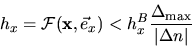 |
(3.22) |
where  is the spacing in the direction of the x-coordinate axis of
the background mesh and
is the spacing in the direction of the x-coordinate axis of
the background mesh and  is
is
 .
.
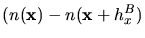
The aim to accurately discretize the solution quantities or to choose a
control function which depends on the solution itself leads
to the problem that the required element size is not known a priori.
A previous simulation mesh with an existing solution must be used as
a background mesh to judge whether or not the mesh density needs to be
increased. There exists no knowledge of how pronounced this increase should
be. A solution dependent measure
 must be defined to assess the existing mesh. To achieve an anisotropic mesh
spacing this metric
must be defined to assess the existing mesh. To achieve an anisotropic mesh
spacing this metric  must be capable to judge the mesh/solution with
respect to the direction .
Typically, reflects interpolation errors, error estimates, second
order derivatives, and error indicators. Numerous approaches can be found
in literature [17,9,6]
must be capable to judge the mesh/solution with
respect to the direction .
Typically, reflects interpolation errors, error estimates, second
order derivatives, and error indicators. Numerous approaches can be found
in literature [17,9,6]
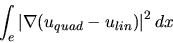 |
(3.23) |
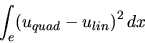 |
(3.24) |
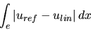 |
(3.25) |
where  denotes a quadratic interpolant,
  a linear
interpolant, and
a linear
interpolant, and  a reference solution.
Error indicators or a posteriori error estimates for
a reference solution.
Error indicators or a posteriori error estimates for  can be
developed if specific properties of the solution, e.g. in the case of
elliptic or parabolic problems, are known [10]. For anisotropic control the error contribution of each edge of the mesh
element must be separately evaluated.
can be
developed if specific properties of the solution, e.g. in the case of
elliptic or parabolic problems, are known [10]. For anisotropic control the error contribution of each edge of the mesh
element must be separately evaluated.
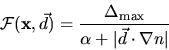
The control function can be formally expressed as
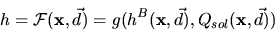 |
(3.26) |
where  is the local mesh spacing of the background mesh.
For some applications, e.g. periodic systems, such an absolute value
for serves as an upper bound to guarantee a certain accuracy.
An explicit function for is also needed for global adaptation.
The entire domain is remeshed with new elements which are not created from
simple refinement of the old elements. The old mesh is used purely as
background mesh providing the old solution and not for the actual
construction of the adapted mesh.
The meshing process guided by a measure becomes an iterative
process which starts on an initial coarse mesh with a first solution.
The initial mesh can only be controlled by geometrical constraints and/or
key variables which are independent of the solution.
However, most practical codes perform a less sophisticated
adaptation. Adaptation usually means then local adaptation by means
of local refinement. The function is not known, instead
threshold decisions based on determine whether or not an element
is locally split in half. The mesh is only adapted isotropically and
locally to the solution.
is the local mesh spacing of the background mesh.
For some applications, e.g. periodic systems, such an absolute value
for serves as an upper bound to guarantee a certain accuracy.
An explicit function for is also needed for global adaptation.
The entire domain is remeshed with new elements which are not created from
simple refinement of the old elements. The old mesh is used purely as
background mesh providing the old solution and not for the actual
construction of the adapted mesh.
The meshing process guided by a measure becomes an iterative
process which starts on an initial coarse mesh with a first solution.
The initial mesh can only be controlled by geometrical constraints and/or
key variables which are independent of the solution.
However, most practical codes perform a less sophisticated
adaptation. Adaptation usually means then local adaptation by means
of local refinement. The function is not known, instead
threshold decisions based on determine whether or not an element
is locally split in half. The mesh is only adapted isotropically and
locally to the solution.
Next: 3.4 Local Adaptation
Up: 3. Mesh Generation
Previous: 3.2.3 Simple, Distinctive Mesh
Peter Fleischmann
2000-01-20