If an arbitrary potential barrier is segmented into N regions with constant
potentials (see Fig. 3.9) the wave function in each region can be written as
the sum of an incident and a reflected wave [93]
 with the wave number
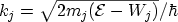 . The wave amplitudes
  ,
,  , the
carrier mass
, the
carrier mass  , and the potential energy
  are assumed constant for
each region
are assumed constant for
each region  . With the interface conditions for energy and momentum
conservation
. With the interface conditions for energy and momentum
conservation
the outgoing wave of a layer relates to the incident wave by a complex
transfer matrix:
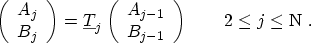 |
(3.75) |
The transfer matrices are of the form
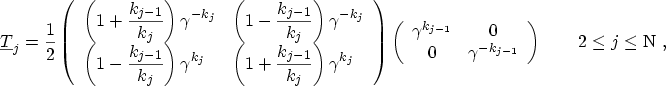 |
(3.76) |
with the phase factor
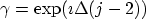 .
The transmitted wave in Region N can then be calculated from the incident
wave by subsequent multiplication of transfer matrices:
.
The transmitted wave in Region N can then be calculated from the incident
wave by subsequent multiplication of transfer matrices:
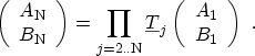 |
(3.77) |
If it is assumed that there is no reflected wave in Region N and the
amplitude of the incident wave is unity, (3.77) simplifies to
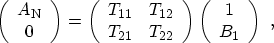 |
(3.78) |
and the transmission coefficient can be calculated from (3.54).
The transfer-matrix method based on constant potential segments has the
obvious shortcoming that, for practical barriers, the accuracy of the
resulting matrix strongly depends on the chosen resolution. A more rigorous
approach is to use linear potential segments.
A. Gehring: Simulation of Tunneling in Semiconductor Devices