3.5.3.2 Piecewise-Linear Potential

A general barrier may consist of several segments with linear potential sandwiched between contact segments where the potential is constant, as depicted in Fig. 3.11. The wave functions within these four regions can be written as (confer (3.67) and (3.68) for a linear potential)

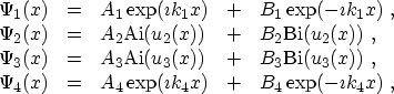$$\begin{array}{rclcl} \Psi_1(x) &=& A_1 \exp(\imath k_1 x) &+&... ... \exp(\imath k_4 x) &+& B_4 \exp(-\imath k_4 x) \ , \end{array}$$ (3.79)

with $u(x)$ from (3.68) and the $x$-independent derivative

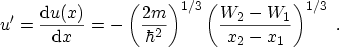$$u' = \frac{\ensuremath {\mathrm{d}}u(x)}{\ensuremath {\mathrm{d}}... ...{2m}{\hbar^2} \right)^{1/3} \left( \frac{W_2 - W_1}{x_2 - x_1}\right)^{1/3} \ .$$ (3.80)

The conditions for continuity of the wave functions and their derivatives yield the following equation system, where abbreviations for the left and right value of $u(x)$ in a layer $\buildrel \leftarrow \over u_j = u_j(l_{j-2})$, $\buildrel \rightarrow \over u_j = u_j(l_{j-1})$, and their derivatives $u_j'$ for $2\leq j \leq \mathrm{N}-1$ have been used.

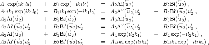$$\begin{array}{lclclcl} A_1 \exp(\imath k_1 l_0) &+& B_1 \exp(... ...2 k_4) &-& B_4 \imath k_4 \exp(-\imath l_2 k_4) \ , \end{array}$$ (3.81)

Figure 3.11: An energy barrier consisting of constant and linear potential segments.

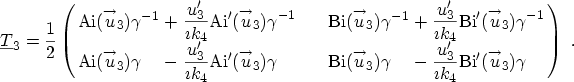
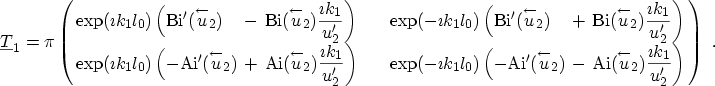
The transfer matrices between adjacent layers are again calculated from (3.75). Using the first two equations of (3.81) and the WRONSKI an^3.8 [138]

$$\mathrm{Wr}\{\ensuremath{\mathrm{Ai}}(z), \ensuremath{\mathrm{Bi}... ...'}}(z) - \ensuremath{\mathrm{Ai'}}(z)\ensuremath{\mathrm{Bi}}(z) = \pi^{-1} \ ,$$ (3.82)

the matrix $\ensuremath{{\underline{T}}}_1$ can be simplified to

$$\ensuremath{{\underline{T}}}_1 = \pi \left( \setlength{\arraycols... ...ver u_2) \displaystyle \frac{\imath k_1}{ u_2' } \right) \end{array} \right)\ .$$

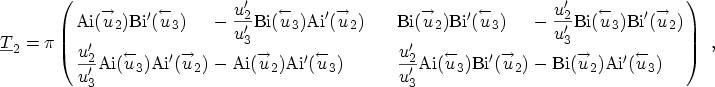
Using the next two lines of (3.81) yields

$$\ensuremath{{\underline{T}}}_2 = \pi \left( \setlength{\arraycols... ...uremath{\mathrm{Ai'}}(\buildrel \leftarrow \over u_3) \\ \end{array} \right)\ ,$$

and the last two equations yield with the phase factor $\gamma = \exp(\imath l_2k_4)$

$$\ensuremath{{\underline{T}}}_3 = \frac{1}{2} \left( \setlength{\a... ...{\mathrm{Bi'}}(\buildrel \rightarrow \over u_3)\gamma \\ \end{array} \right)\ .$$ (3.83)

While being more accurate than the constant potential approach this method is computationally more expensive. This drawback, however, is offset by the fact that a lower resolution and thus fewer matrix multiplications are necessary to resolve an energy barrier consisting of linear potential segments.

Simulations using the transfer-matrix method have been reported by several authors [145,146,147,148]. Others compared the constant and linear potential approaches and found the constant potential method more feasible for device simulation [149]. The main advantage of the linear-potential transfer-matrix method is, that for linear potential segments the accuracy does not depend on the resolution as it does for the constant-potential transfer-matrix method. However, the evaluation of the AIRY functions must be carefully implemented to avoid overflow.

Although the transfer-matrix method for constant or linear potential segments is intuitively easy to understand and implement, the main shortcoming of the method is that it becomes numerically instable for thick barriers. This has been observed by several authors [150,151,152,153,149]. The reason for the numerical problems is that during the matrix multiplications exponentially growing and decaying states have to be multiplied, leading to rounding errors which eventually exceed the amplitude of the wave function itself for thick barriers.

These problems have been overcome by a further segmentation of the barrier into slices with more accurate transfer matrices [150], the use of scattering matrices instead of transfer matrices [151], iterative methods [152], or by simply setting the transfer matrix entries to zero if the decay factor $\sum k_j x_j$ exceeds a certain value of about 20 [149]. In the next section a method will be presented which avoids this problem and allows a fast and reliable transmission coefficient estimation.

A. Gehring: Simulation of Tunneling in Semiconductor Devices