3.6.2 Eigenvalues of Arbitrary Energy Wells

To calculate the eigenvalues of an arbitrary energy well it is necessary to solve SCHRÖDINGER's equation. This can be done using the method of finite differences. It is based on a discretization of the HAMILTONian on a spatial grid and given by (3.84) which is repeated here for convenience

$$\ensuremath{{\underline{H}}}\Psi_j = -s_j\Psi_{j-1} + d_j\Psi_j - s_{j+1}\Psi_{j+1} = {\mathcal{E}}\Psi_j \ .$$

While in Section 3.5.4, a constant value of the electron mass in the simulated region was used, a discretization which allows for a position-dependent carrier mass reads

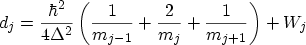$$d_j = \frac{\hbar^2}{4\Delta^2} \left( \frac{1}{m_{j-1}} + \frac{2}{m_{j}} + \frac{1}{m_{j+1}} \right) + W_j$$ (3.101)

and

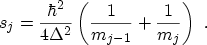$$s_j = \frac{\hbar^2}{4\Delta^2} \left( \frac{1}{m_{j-1}} + \frac{1}{m_{j}} \right) \ .$$ (3.102)

The system HAMILTONian is tridiagonal and, for a six-point example, can be written similar to (3.91) but without the entries for $\zeta$ and $\xi$:

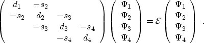$$\left( \begin{array}{ccccc} d_1 & -s_2 \\ -s_2 & d_2 & -s_3 \\ & ... ...begin{array}{c} \Psi_1 \\ \Psi_2 \\ \Psi_3 \\ \Psi_4 \\ \end{array} \right) \ .$$ (3.103)

The values $\Psi_0$ and $\Psi_5$ must be 0 in this case, that is closed boundary conditions are assumed. The system HAMILTONian is real and symmetric, therefore all eigenvalues are real. While this matrix equation looks similar to (3.91), there are important differences. Here it is necessary to solve the eigenvalue equation to get a value for ${\mathcal{E}}_i$ and $\Psi_i$. In (3.91), any value of ${\mathcal{E}}$ leads to a valid solution for $\Psi_i$, and the solution is obtained by solving a complex equation system.

A. Gehring: Simulation of Tunneling in Semiconductor Devices