3.7 Compact Tunneling Models
The above presented models for the calculation of tunneling currents require a
considerable computational effort. However, for practical device simulation,
it is desirable to use compact models which do not require large computational
resources. That may be necessary for a quick estimation of the dielectric
thickness from IV data or to predict the impact of gate leakage on the
performance of CMOS
circuits [178,179,180,181,182,183]. The most
frequently used model to describe tunneling is the FOWLER-NORDHEIM formula [184]
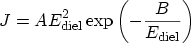 |
(3.117) |
which was originally used to describe tunneling between metals under intense
electric fields. The parameters  and
and  have been refined by
LENZLINGER and SNOW [185]:
have been refined by
LENZLINGER and SNOW [185]:
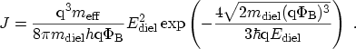 |
(3.118) |
This expression can be derived from the TSU-ESAKI formula (3.13) by
the assumption of zero temperature, a triangular energy barrier, and equal
materials on both sides of the dielectric (the derivation is shown in
Appendix A). Thus, it is not valid for direct tunneling where
the barrier is of trapezoidal shape. Furthermore,
 denotes the
difference between the FERMI energy in the electrode and the conduction
band edge in the dielectric, and not the conduction band offset, as it is
often found in the literature.
denotes the
difference between the FERMI energy in the electrode and the conduction
band edge in the dielectric, and not the conduction band offset, as it is
often found in the literature.
SCHUEGRAF and HU derived correction terms for this
expression to make it applicable to the regime of direct
tunneling [186]
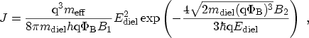 |
(3.119) |
with the correction terms  and
and  given as (the derivation can also be
found in Appendix A)
given as (the derivation can also be
found in Appendix A)
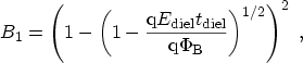 |
(3.120) |
and
 |
(3.121) |
For a triangular barrier the correction factors become  and the
expression simplifies to (3.118). Note that using these equations,
the minimum tunneling current occurs for
and the
expression simplifies to (3.118). Note that using these equations,
the minimum tunneling current occurs for
 V/m which, for a work
function difference
V/m which, for a work
function difference  , does not occur at the minimum applied bias.
A. Gehring: Simulation of Tunneling in Semiconductor Devices