2.3.2.2 Macroscopic Relaxation Time Approximation

The collision term on the right hand side of eqns. (2.53) and (2.54), which represents the various scattering processes, can be 
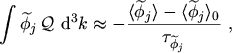
deliberately modeled as

$\displaystyle \ensuremath{\int \ensuremath{\widetilde{\phi}}_j \, \mathcal{Q} \...
...ath{\widetilde{\phi}}_j \rangle}_0}{\tau_{\ensuremath{\widetilde{\phi}}_j}} \ ,$ (2.70)

which is commonly termed as relaxation time approximation [14, p.144]. This equation implies that the perturbed distribution function will relax exponentially to the equilibrium function with one time constant $ \tau_{\ensuremath{\widetilde{\phi}}_j}$ when the perturbing field is removed. A discussion on the validity of this approximation is given in [20, p.139].

The equilibrium distribution function $ f_0(\ensuremath{\boldsymbol{\mathrm{k}}})$ is a symmetric function. Since the even weight functions are symmetric in $ \ensuremath{\boldsymbol{\mathrm{k}}}$ and the odd weight functions are anti-symmetric in $ \ensuremath{\boldsymbol{\mathrm{k}}}$, only the even moments of the equilibrium distribution function will be non-zero whereas the odd moments will vanish

$\displaystyle \ensuremath{\langle \phi_j \rangle}_0$ $\displaystyle = \ensuremath{\int \phi_j(k) \, f_0(k) \,\, \ensuremath{\mathrm{d}}^3 k}$   $\displaystyle \neq 0 \textcolor{lightgrey}{.......}\textrm{for even $j$} \ ,$ (2.71)
$\displaystyle \ensuremath{\langle \ensuremath{\boldsymbol{\mathrm{\phi}}}_j \rangle}_0$ $\displaystyle = \ensuremath{\int \ensuremath{\boldsymbol{\mathrm{\phi}}}_j(\ens...
... \, f_0(\ensuremath{\boldsymbol{\mathrm{k}}}) \,\, \ensuremath{\mathrm{d}}^3 k}$   $\displaystyle = 0 \textcolor{lightgrey}{.......}\textrm{for odd $j$} \ .$ (2.72)

Applying the relaxation time approximation and inserting the calculated gradients from the previous section into eqns. (2.53) and (2.54) leads to the equation set

  $\displaystyle \phi_0:$ $\displaystyle \textcolor{lightgrey}{.......}$ $\displaystyle \ensuremath{\partial_{t} \, \ensuremath{\langle 1 \rangle}}$   $\displaystyle + \ensuremath{\ensuremath{\ensuremath{\boldsymbol{\mathrm{\nabla}...
...remath{\cdot}\ensuremath{\langle \ensuremath{\boldsymbol{\mathrm{v}}} \rangle}}$       $\displaystyle =$   $\displaystyle - R \ ,$ (2.73)
  $\displaystyle \phi_2:$ $\displaystyle \textcolor{lightgrey}{.......}$ $\displaystyle \ensuremath{\partial_{t} \, \ensuremath{\langle \mathcal{E} \rangle}}$   $\displaystyle + \ensuremath{\ensuremath{\ensuremath{\boldsymbol{\mathrm{\nabla}...
...nsuremath{\langle \ensuremath{\boldsymbol{\mathrm{v}}} \, \mathcal{E} \rangle}}$   $\displaystyle + \mathrm{q}\, \ensuremath{\boldsymbol{\mathrm{E}}}\ensuremath{\cdot}\ensuremath{\langle \ensuremath{\boldsymbol{\mathrm{v}}} \rangle}$   $\displaystyle = - \frac{\ensuremath{\langle \mathcal{E} \rangle}- \ensuremath{\langle \mathcal{E} \rangle}_0}{\tau_\mathcal{E}}$   $\displaystyle + G_{\mathcal{E}\, n} \ ,$ (2.74)
  $\displaystyle \phi_4:$ $\displaystyle \textcolor{lightgrey}{.......}$ $\displaystyle \ensuremath{\partial_{t} \, \ensuremath{\langle v^2 \, \mathcal{E} \rangle}}$   $\displaystyle + \ensuremath{\ensuremath{\ensuremath{\boldsymbol{\mathrm{\nabla}...
...th{\langle \ensuremath{\boldsymbol{\mathrm{v}}} \, v^2 \, \mathcal{E} \rangle}}$   $\displaystyle + \frac{4 \, \mathrm{q}}{m} \, \ensuremath{\boldsymbol{\mathrm{E}...
...ensuremath{\langle \ensuremath{\boldsymbol{\mathrm{v}}} \, \mathcal{E} \rangle}$   $\displaystyle = - \frac{\ensuremath{\langle v^2 \, \mathcal{E} \rangle}- \ensuremath{\langle v^2 \, \mathcal{E} \rangle}_0}{\tau_\beta}$   $\displaystyle + G_{\beta \, n} \ ,$ (2.75)

  $\displaystyle \ensuremath{\boldsymbol{\mathrm{\phi}}}_1:$ $\displaystyle \textcolor{lightgrey}{.......}$ $\displaystyle \ensuremath{\ensuremath{\ensuremath{\boldsymbol{\mathrm{\nabla}}}...
...\mathrm{v}}} \ensuremath{\otimes}\ensuremath{\boldsymbol{\mathrm{p}}} \rangle}}$   $\displaystyle + \mathrm{q}\, \ensuremath{\boldsymbol{\mathrm{E}}}\ensuremath{\cdot}\ensuremath{\langle \ensuremath{\widetilde{\delta}} \rangle}$   $\displaystyle = - \frac{\ensuremath{\langle \ensuremath{\boldsymbol{\mathrm{p}}} \rangle}}{\tau_m} \ ,$ (2.76)
  $\displaystyle \ensuremath{\boldsymbol{\mathrm{\phi}}}_3:$ $\displaystyle \textcolor{lightgrey}{.......}$ $\displaystyle \ensuremath{\ensuremath{\ensuremath{\boldsymbol{\mathrm{\nabla}}}...
...nsuremath{\otimes}\ensuremath{\boldsymbol{\mathrm{v}}} \, \mathcal{E} \rangle}}$   $\displaystyle + \mathrm{q}\, \ensuremath{\boldsymbol{\mathrm{E}}}\ensuremath{\c...
...{\mathrm{v}}} \ensuremath{\otimes}\ensuremath{\boldsymbol{\mathrm{v}}} \rangle}$   $\displaystyle = - \frac{\ensuremath{\langle \ensuremath{\boldsymbol{\mathrm{v}}} \, \mathcal{E} \rangle}}{\tau_S} \ ,$ (2.77)
  $\displaystyle \ensuremath{\boldsymbol{\mathrm{\phi}}}_5:$ $\displaystyle \textcolor{lightgrey}{.......}$ $\displaystyle \ensuremath{\ensuremath{\ensuremath{\boldsymbol{\mathrm{\nabla}}}...
...th{\otimes}\ensuremath{\boldsymbol{\mathrm{v}}} \, v^2 \, \mathcal{E} \rangle}}$   $\displaystyle + \frac{\mathrm{q}}{m} \, \ensuremath{\boldsymbol{\mathrm{E}}}\en...
...\mathrm{v}}} \ensuremath{\otimes}\ensuremath{\boldsymbol{\mathrm{v}}}) \rangle}$   $\displaystyle = - \frac{\ensuremath{\langle \ensuremath{\boldsymbol{\mathrm{v}}} \, v^2 \, \mathcal{E} \rangle}}{\tau_K} \ ,$ (2.78)

where $ \tau_m$, $ \tau_\mathcal{E}$, $ \tau_S$, $ \tau_\beta$, $ \tau_K$ are the relaxation times for momentum, energy, energy flux density, kurtosis, and kurtosis flux density, respectively.

M. Gritsch: Numerical Modeling of Silicon-on-Insulator MOSFETs PDF