2.3.3.1 Maxwell Distribution

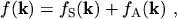
To close the system of equations an a priori assumption about the shape of the distribution function can be made. A shifted MAXWELL distribution function is a frequently used ansatz

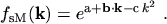$$f_\mathrm{sM}(\ensuremath{\boldsymbol{\mathrm{k}}}) = e^{\mathrm{... ...}\ensuremath{\cdot}\ensuremath{\boldsymbol{\mathrm{k}}}- \mathrm{c} \, k^2} \ .$$ (2.105)

Every distribution function can be seen as being comprised of a symmetric and an anti-symmetric part

$$f(\ensuremath{\boldsymbol{\mathrm{k}}}) = f_\mathrm{S}(\ensuremat... ...ldsymbol{\mathrm{k}}}) + f_\mathrm{A}(\ensuremath{\boldsymbol{\mathrm{k}}}) \ ,$$ (2.106)

whereby the two parts satisfy the following relations

$$f_\mathrm{S}(\ensuremath{\boldsymbol{\mathrm{k}}}) = f_\mathrm{S}(- \ensuremath{\boldsymbol{\mathrm{k}}}) = \frac{1}{2} \, \bigl(f(\ensuremath{\boldsymbol{\mathrm{k}}}) + f(- \ensuremath{\boldsymbol{\mathrm{k}}}) \bigr) \ ,$$ (2.107)

$$f_\mathrm{A}(\ensuremath{\boldsymbol{\mathrm{k}}}) = - f_\mathrm{A}(- \ensuremath{\boldsymbol{\mathrm{k}}}) = \frac{1}{2} \, \bigl(f(\ensuremath{\boldsymbol{\mathrm{k}}}) - f(- \ensuremath{\boldsymbol{\mathrm{k}}}) \bigr) \ .$$ (2.108)

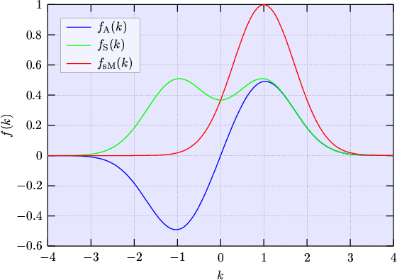
An example of a shifted MAXWELLian distribution function together with its symmetric and anti-symmetric part is depicted in Fig. 2.1.

Figure 2.1: Shape of a shifted MAXWELL distribution function $f_\textrm {sM}(k)$ and its symmetric $f_\textrm {S}(k)$ and anti-symmetric $f_\textrm {A}(k)$ parts. The displacement is assumed to be large.

The diffusion approximation now assumes that the displacement of the distribution function is small which means that the anti-symmetric part is much smaller than the symmetric one. Then it is justified to approximate the shifted MAXWELL distribution function by a series expansion with respect to the displacement and to truncate the expansion after the first term:

$$f(\ensuremath{\boldsymbol{\mathrm{k}}}) = e^{\mathrm{a} + \ensuremath{\boldsymbol{\mathrm{b}}}\ensuremath{\cdot}\ensuremath{\boldsymbol{\mathrm{k}}}- \mathrm{c} \, k^2}$$ (2.109)

$$= e^{\mathrm{a} - \mathrm{c} \, k^2} \, e^{\ensuremath{\boldsymbol{\mathrm{b}}}\ensuremath{\cdot}\ensuremath{\boldsymbol{\mathrm{k}}}}$$ (2.110)

$$\approx f_\mathrm{M}(\vert\ensuremath{\boldsymbol{\mathrm{k}}}\ve... ...dsymbol{\mathrm{b}}}\ensuremath{\cdot}\ensuremath{\boldsymbol{\mathrm{k}}}) \ .$$ (2.111)

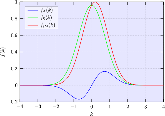
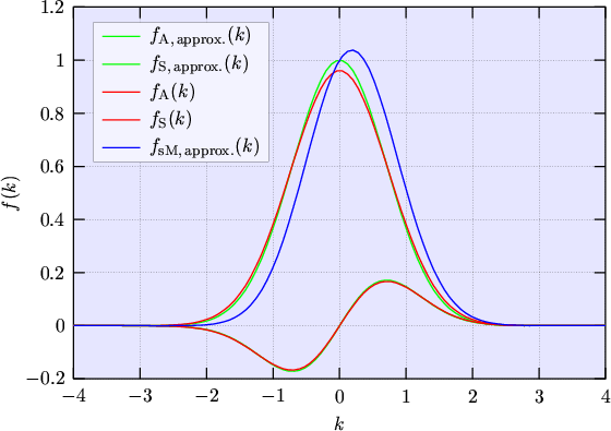
A decomposition of a shifted MAXWELLian distribution function, where the displacement is small, is depicted in Fig. 2.2. The symmetric and anti-symmetric part from Fig. 2.2 together with their approximations are depicted in Fig. 2.3. As can be seen, if the displacement is small the diffusion approximation is well justified.

Figure 2.2: Shape of a shifted MAXWELL distribution function $f_\textrm {sM}(k)$ and its symmetric $f_\textrm {S}(k)$ and anti-symmetric $f_\textrm {A}(k)$ parts. The displacement is assumed to be small.

Figure 2.3: Symmetrical $f_\textrm {S}(k)$ and anti-symmetric $f_\textrm {A}(k)$ parts of a shifted MAXWELL distribution function in comparison with the result of the diffusion approximation.

The interpretation of eqn. (2.111) is that the symmetric part can be approximated by a non-displaced MAXWELL distribution function

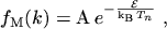$$f_\mathrm{M}(k) = \mathrm{A}\, e^{ - \frac{\mathcal{E}}{\mathrm{k}_\mathrm{B}\, T_n}} \ ,$$ (2.112)

and the anti-symmetric part by a non-displaced MAXWELL distribution function multiplied by $\ensuremath{\boldsymbol{\mathrm{b}}} \ensuremath{\cdot}\ensuremath{\boldsymbol{\mathrm{k}}}$.

For closing the moment equation system at even moments, an assumption about the symmetric part of the distribution function must be introduced since the integrals of even powers of $\ensuremath{\boldsymbol{\mathrm{k}}}$ multiplied with the anti-symmetric part vanish. Vice versa, for closing the moment equation system at odd moments, only the anti-symmetric part of the distribution function must be assumed since the integrals of odd powers of $\ensuremath{\boldsymbol{\mathrm{k}}}$ multiplied with the symmetric part vanish.

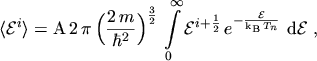
The even moments will be calculated as powers of the energy $\mathcal{E}^i$ since for parabolic bands $\ensuremath{\langle v^2 \, \mathcal{E} \rangle}$ and $\ensuremath{\langle \mathcal{E}^2 \rangle}$ only differ by a constant prefactor $m / 2$. The same holds true for $\ensuremath{\langle v^4 \, \mathcal{E} \rangle}$ and $\ensuremath{\langle \mathcal{E}^3 \rangle}$ where the constant prefactor yields $m^2 / 4$. Starting from

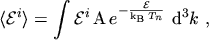$$\ensuremath{\langle \mathcal{E}^i \rangle}= \ensuremath{\int \mat... ...\mathcal{E}}{\mathrm{k}_\mathrm{B}\, T_n}} \,\, \ensuremath{\mathrm{d}}^3 k}\ ,$$ (2.113)

the integration over $\ensuremath{\boldsymbol{\mathrm{k}}}$-space is performed in spherical polar coordinates using the transformation

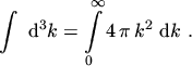$$\ensuremath{\int \,\, \ensuremath{\mathrm{d}}^3 k}= \ensuremath{\int_0^{\infty} 4 \, \pi \, k^2 \,\, \ensuremath{\mathrm{d}}k}\ .$$ (2.114)

Assuming a parabolic dispersion relation, $\mathcal{E}= \frac{\hbar^2 \, k^2}{2 \, m}$, eqn. (2.113) becomes

$$\ensuremath{\langle \mathcal{E}^i \rangle}= \mathrm{A}\, 2 \, \pi... ...l{E}}{\mathrm{k}_\mathrm{B}\, T_n}} \,\, \ensuremath{\mathrm{d}}\mathcal{E}}\ ,$$ (2.115)

and making the substitution $\mathcal{E}= \mathrm{k}_\mathrm{B}\, T_n \, u$ eqn. (2.115) can be written in a form suitable for making use of the gamma function

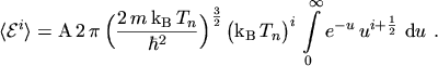$$\ensuremath{\langle \mathcal{E}^i \rangle}= \mathrm{A}\, 2 \, \pi... ...nt_0^{\infty} e^{ - u} \, u^{i + \frac{1}{2}} \,\, \ensuremath{\mathrm{d}}u}\ .$$ (2.116)

Using the gamma function and its identity rules

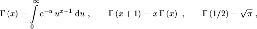$$\ensuremath{\Gamma \left( x \right) }= \ensuremath{\int_0^{\infty... ...or{lightgrey}{.......}\ensuremath{\Gamma \left( 1 / 2 \right) }= \sqrt{\pi} \ ,$$ (2.117)

transforms the even moments of the MAXWELL distribution function to

$$\ensuremath{\langle \mathcal{E}^i \rangle}= \mathrm{A}\, 2 \, \pi... ...igr)^i \, \Bigl(i + \frac{1}{2}\Bigr) \, \Gamma \Bigl(i + \frac{1}{2}\Bigr) \ .$$ (2.118)

By normalizing the distribution function to $\ensuremath{\langle 1 \rangle} \overset{!}{=} n$ the coefficient $\mathrm{A}$ can be evaluated. Calculating the moments is then straightforward and yields

$$\ensuremath{\langle \mathcal{E}^0 \rangle}_\mathrm{M} = n \ ,$$ (2.119)

$$\ensuremath{\langle \mathcal{E}^1 \rangle}_\mathrm{M} = n \, \frac{3}{2} \, \mathrm{k}_\mathrm{B}\, T_n \ ,$$ (2.120)

$$\ensuremath{\langle \mathcal{E}^2 \rangle}_\mathrm{M} = n \, \frac{5 \ensuremath{\cdot}3} {2 \ensuremath{\cdot}2} \, \bigl(\mathrm{k}_\mathrm{B}\, T_n\bigr)^2 \ ,$$ (2.121)

$$\ensuremath{\langle \mathcal{E}^3 \rangle}_\mathrm{M} = n \, \frac{7 \ensuremath{\cdot}5 \ensuremath{\cdot}3} {2 \ensur... ...h{\cdot}2 \ensuremath{\cdot}2} \, \bigl(\mathrm{k}_\mathrm{B}\, T_n\bigr)^3 \ ,$$ (2.122)

or by using the weight functions (2.45) to (2.48)

$$\ensuremath{\langle \phi_0 \rangle}_\mathrm{M} = n \ ,$$ (2.123)

$$\ensuremath{\langle \phi_2 \rangle}_\mathrm{M} = \frac{3}{2} \, \mathrm{k}_\mathrm{B}\, n \, T_n \ ,$$ (2.124)

$$\ensuremath{\langle \phi_4 \rangle}_\mathrm{M} = \frac{5 \ensuremath{\cdot}3}{2} \, \frac{\mathrm{k}_\mathrm{B}^2}{m} \, n \, T_n^2 \ ,$$ (2.125)

$$\ensuremath{\langle \phi_6 \rangle}_\mathrm{M} = \frac{7 \ensuremath{\cdot}5 \ensuremath{\cdot}3}{2} \, \frac{\mathrm{k}_\mathrm{B}^3} {m^2} \, n \, T_n^3 \ .$$ (2.126)

M. Gritsch: Numerical Modeling of Silicon-on-Insulator MOSFETs PDF