|
|
|
|
Previous: 2.3.3.1 Maxwell Distribution Up: 2.3.3 Closure Next: 2.3.3.3 Drift-Diffusion Transport Model - Closure at |
|
|
|
|
Previous: 2.3.3.1 Maxwell Distribution Up: 2.3.3 Closure Next: 2.3.3.3 Drift-Diffusion Transport Model - Closure at |
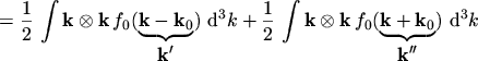
Let now be ![]() a shifted distribution function
a shifted distribution function
| (2.127) |
| (2.128) | ||
| (2.129) | ||
| (2.130) |
As has already been shown in eqns. (2.106) to (2.108),
every function can be split into its symmetric and its anti-symmetric part. Since the weight
functions
![]() and
and
![]() are even functions, only
the symmetric part of the distribution function has to be taken into account
are even functions, only
the symmetric part of the distribution function has to be taken into account
Eqn. (2.131) is now used in the evaluation of the statistical
average
![]() :
:
The statistical average of
![]() can be evaluated in the same way
yielding
can be evaluated in the same way
yielding
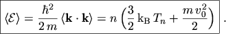
For a MAXWELL distribution the first term of the RHS of eqn. (2.133) has already been calculated as eqn. (2.120). Therefore eqn. (2.133) can be written as
As can be seen, without the diffusion approximation the average carrier energy is composed of
a thermal component and a kinetic2.8 component.
A consequence of the diffusion approximation is that the kinetic term is neglected
[24, p.71] [25, p.736]. By assuming
![]() ,
,
![]() , and
, and
![]() for electrons
in silicon [9, p.191] the ratio
for electrons
in silicon [9, p.191] the ratio
![]() yields
yields
![]() . However, in reality this ratio is much bigger because in the regions, where the
assumed electron saturation velocity is reached, the electron temperature is much higher than
the lattice temperature [26, p.34]. Neglecting the kinetic term appears
therefore justified. Note that simulations at very low temperatures would have to include
this term. Under dynamic conditions this term can also be significant
[27, p.413].
. However, in reality this ratio is much bigger because in the regions, where the
assumed electron saturation velocity is reached, the electron temperature is much higher than
the lattice temperature [26, p.34]. Neglecting the kinetic term appears
therefore justified. Note that simulations at very low temperatures would have to include
this term. Under dynamic conditions this term can also be significant
[27, p.413].
The first term of the RHS of eqn. (2.132) has also already been calculated as eqn. (2.88). Eqn. (2.132) can therefore be written as
By calculating the statistical average
![]()
| (2.137) |
| (2.138) |
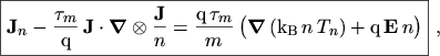
Inserting eqn. (2.139) into eqn. (2.136) yields the final form of the current relation
The importance of this additional term within semiconductor equations is controversial. Phenomena known from fluid dynamics like super-sonic transport and propagation of electron shock-waves arise [29] [30]. The resulting transport model is referred to as (full) hydrodynamic transport model2.9.
M. Gritsch: Numerical Modeling of Silicon-on-Insulator MOSFETs PDF