2.3.3.4 Energy Transport Model - Closure at
 and
and 
By taking the first three moments of BOLTZMANN's transport equation, eqns. (2.99),
(2.100), and (2.102), into account
 |
(2.149) |
an energy transport model is obtained. To close the system the moment of third order
 must be evaluated. This is the only case where we close at an odd
moment. For this the anti-symmetric part eqn. (2.111) has to be used.
The coefficient
must be evaluated. This is the only case where we close at an odd
moment. For this the anti-symmetric part eqn. (2.111) has to be used.
The coefficient
 found in eqn. (2.111) is determined from the
first moment. Since odd moments are calculated, only the anti-symmetric part of the
distribution function yields moments different from zero.
found in eqn. (2.111) is determined from the
first moment. Since odd moments are calculated, only the anti-symmetric part of the
distribution function yields moments different from zero.
Using this closure the 3-moments energy transport model becomes
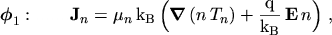
The expression for the energy flux density eqn. (2.155) describes pure heat convection. It
is often empirically extended by a conductive term where FOURIER's law is used for
the heat flow
 [36]
[36]
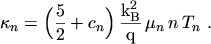
The thermal conductivity  is calculated by the WIEDEMANN-FRANZ law, and
is proportional to the mobility
is calculated by the WIEDEMANN-FRANZ law, and
is proportional to the mobility  and the carrier temperature
 |
(2.158) |
Care must be taken to perform this extension in a consistent way.  has to be set to zero
since the prefactor in eqn. (2.155) reads
has to be set to zero
since the prefactor in eqn. (2.155) reads
 . In the literature this is often
found inconsistent [37].
. In the literature this is often
found inconsistent [37].
However, the heat flow term comes naturally into existence when the first four moment
eqns. (2.99), (2.100),
(2.102), and (2.103) are taken into account
Together with the closure relation derived from a heated MAXWELLian,
eqn. (2.125),
 |
(2.163) |
the resulting energy transport model reads
In contrast to the drift-diffusion transport model the thermal diffusion current is included in
eqn. (2.165) since the gradient operates on both  and . Moreover, the
velocity overshoot effect is included in this equation set since depends on ,
which in turn depends via eqns. (2.166) and (2.167)
in a non-local manner on the electric field distribution.
and . Moreover, the
velocity overshoot effect is included in this equation set since depends on ,
which in turn depends via eqns. (2.166) and (2.167)
in a non-local manner on the electric field distribution.
As already mentioned, the heat flow term is present in this model and the
WIEDEMANN-FRANZ law for is obtained consistently.
Eqn. (2.166) represents the standard form of a conservation equation.
The left-hand side represents the energy outflow from some control volume, which must be equal
to the sum of the rate of change of the energy density, the energy delivered to the carriers
by the electric field per unit volume and time, and the rate of change of energy density due
to collisions.
Using an energy transport model, non-local effects like the velocity overshoot are covered.
Interestingly, this model also predict a velocity overshoot when the electric field decreases
rapidly, for instance at the end of a channel in a MOS transistor. This velocity
overshoot is not observed in the more rigorous Monte Carlo simulations and thus termed
spurious velocity overshoot. However, it is generally believed that the influence of
this effect on device characteristics is small. It appears that the spurious velocity
overshoot is a result of the truncation of the moment expansion of BTE at a certain
order and close the equation system by some empirical expression. A second point is, that the
relaxation times are not single valued functions of the energy. Due to these two reasons it
is believed that the spurious velocity overshoot can never be completely eliminated using a
finite number of moment equations. More detailed investigations can be found in
[38].
M. Gritsch: Numerical Modeling of Silicon-on-Insulator MOSFETs PDF