3.3.2.2 Flux Equations

The current density is discretized by a scheme which is frequently referred to as SCHARFETTER-GUMMEL discretization [51]. The extension of the discretization to the flux equations stemming from the higher order moments of BOLTZMANN's equation is not beyond controversy, so different approaches can be found in the literature. In [23] it is assumed that the electron concentration is a known function of exponential shape. This strategy is refined in [37] where the variation of the electron concentration obtained from the discretization of the current density equation is used for discretizing the energy flux density. This text will follow the approach presented in [31], which is an extension of [52] and [53], where a generalized expression for the fluxes is used and no assumption about the variation of the carrier concentration is made.

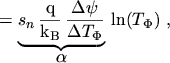
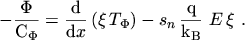
By rewriting the flux equations (2.188) to (2.190)

$$\ensuremath{\boldsymbol{\mathrm{J}}}_n = - \mathrm{C}_1 \, \Bigl( \ensuremath{\ensuremath{\ensuremath{\boldsymbol{\mathrm{\nabla}}}}\, (n \, T_n)} - s_n \, \frac{\mathrm{q}}{\mathrm{k}_\mathrm{B}} \, \ensuremath{\boldsymbol{\mathrm{E}}}\, (n \, T_n) \, \frac{1}{T_n} \Bigr) \ ,$$ (3.34)

$$\ensuremath{\boldsymbol{\mathrm{S}}}_n = - \mathrm{C}_3 \, \Bigl( \ensuremath{\ensuremath{\ensuremath{\boldsymbol{\mathrm{\nabla}}}}\, (n \, T_n^2 \, \beta_n)} - s_n \, \frac{\mathrm{q}}{\mathrm{k}_\mathrm{B}} \, \ensuremath{... ...l{\mathrm{E}}}\, (n \, T_n^2 \, \beta_n) \, \frac{1}{T_n \, \beta_n} \Bigr) \ ,$$ (3.35)

$$\ensuremath{\boldsymbol{\mathrm{K}}}_n = - \mathrm{C}_5 \, \Bigl( \ensuremath{\ensuremath{\ensuremath{\boldsymbol{\mathrm{\nabla}}}}\, (n \, T_n^3 \, \beta_n^3)} - s_n \, \frac{\mathrm{q}}{\mathrm{k}_\mathrm{B}} \, \ensuremath{... ...athrm{E}}}\, (n \, T_n^3 \, \beta_n^3) \, \frac{1}{T_n \, \beta_n^2} \Bigr) \ ,$$ (3.36)

a common functional form can be recognized. Therefore a general flux equation is introduced

$$\ensuremath{\boldsymbol{\mathrm{\Phi}}}= - \mathrm{C}_\Phi \, \Bi... ...emath{\boldsymbol{\mathrm{E}}}\, (\xi \, T_\Phi) \, \frac{1}{T_\Phi} \Bigr) \ .$$ (3.37)

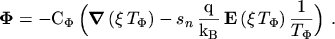
The meanings of the generalized density $\xi$ and temperature $T_\Phi$ is found by inspection:

$$\ensuremath{\boldsymbol{\mathrm{J}}}_n : \qquad \xi = n \ , \textcolor{lightgrey}{.......}T_\Phi = T_n \ ,$$ (3.38)

$$\ensuremath{\boldsymbol{\mathrm{S}}}_n : \qquad \xi = n \, T_n \ , \textcolor{lightgrey}{.......}T_\Phi = T_n \, \beta_n \ ,$$ (3.39)

$$\ensuremath{\boldsymbol{\mathrm{K}}}_n : \qquad \xi = n \, T_n^2 \, \beta_n \ , \textcolor{lightgrey}{.......}T_\Phi = T_n \, \beta_n^2 \ .$$ (3.40)

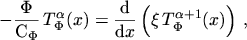
By projecting eqn. (3.37) onto a grid line a one-dimensional differential equation is obtained

$$- \frac{\Phi}{\mathrm{C}_\Phi} = \ensuremath{\frac{\ensuremath{\m... ...xi \, T_\Phi)}- s_n \, \frac{\mathrm{q}} {\mathrm{k}_\mathrm{B}} \ E \, \xi \ .$$ (3.41)

To solve this equation the following assumptions have been made:

• constant general flux $\Phi$,
• constant electric field

  $$E = - \frac{\Delta \psi}{\Delta x} \ ,$$ (3.42)

  
  

• linear variation of the general temperature $T_\Phi$

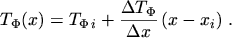  $$T_\Phi(x) = T_{\Phi \, i} + \frac{\Delta T_\Phi}{\Delta x} \, (x - x_i) \ .$$ (3.43)

  
  

The solution of eqn. (3.41) is found by multiplication with an integrating factor $w(x)$ and by sub-sequentially comparing the coefficients of the resulting equation with the total derivative of the product $(\xi \, T_\Phi) \, w(x)$:

$$- \frac{\Phi}{\mathrm{C}_\Phi} \, w(x) = \ensuremath{\frac{\ensuremath{\mathrm{d}}}{\ensuremath{\mathrm{... ...mathrm{d}}}{\ensuremath{\mathrm{d}}x} \, \Bigl( (\xi \, T_\Phi) \, w(x) \Bigr)}$$ (3.44)

$$= \ensuremath{\frac{\ensuremath{\mathrm{d}}}{\ensuremath{\mathrm{... ...\, \ensuremath{\frac{\ensuremath{\mathrm{d}}w(x)}{\ensuremath{\mathrm{d}}x}}\ .$$ (3.45)

Comparing the coefficients leads to

$$T_\Phi \, \ensuremath{\frac{\ensuremath{\mathrm{d}}w}{\ensuremath{\mathrm{d}}x}} = - s_n \, \frac{\mathrm{q}}{\mathrm{k}_\mathrm{B}} \, E \, w \ ,$$ (3.46)

$$\frac{1}{w} \, \ensuremath{\frac{\ensuremath{\mathrm{d}}w}{\ensuremath{\mathrm{d}}x}} = - s_n \, \frac{\mathrm{q}}{\mathrm{k}_\mathrm{B}} \, \frac{E}{T_\Phi(x)} \ .$$ (3.47)

This equation can be solved for the integrating factor $w$, taking into account the assumptions (3.42) and (3.43):

$$\ln(w) = \underbrace{s_n \, \frac{\mathrm{q}}{\mathrm{k}_\mathrm{B}} \, \frac{\Delta \psi} {\Delta T_\Phi}}_{\textstyle \alpha} \, \ln(T_\Phi) \ ,$$ (3.48)

$$w(x) = T_\Phi^\alpha(x) \ , \textcolor{lightgrey}{.......}\alpha = s_n... ...rac{\mathrm{q}}{\mathrm{k}_\mathrm{B}} \, \frac{\Delta \psi}{\Delta T_\Phi} \ .$$ (3.49)

Inserting the integrating factor into eqn. (3.44)

$$- \frac{\Phi}{\mathrm{C}_\Phi} \, T_\Phi^\alpha(x) = \ensuremath{... ...}}{\ensuremath{\mathrm{d}}x} \, \Bigl( \xi \, T_\Phi^{\alpha + 1}(x) \Bigr)}\ ,$$ (3.50)

and assuming that the flux $\Phi$ is constant between two grid points, eqn. (3.50) can be integrated from $x_i$ to $x_j$

$$- \frac{\Phi}{\mathrm{C}_\Phi} \, \frac{T_\Phi^{\alpha + 1}}{\alpha + 1} \biggr\vert _{x_i}^{x_j} \, \frac{\Delta x}{\Delta T_\Phi} = \xi \, T_\Phi^{\alpha + 1} \biggr\vert _{x_i}^{x_j} \ ,$$ (3.51)

$$- \frac{\Phi}{\mathrm{C}_\Phi} \, \frac{\Delta x}{(\alpha + 1) \,... ..._\Phi} \, \Bigl( T_{\Phi \, j}^{\alpha + 1} - T_{\Phi \, i}^{\alpha + 1} \Bigr) = \xi_j \, T_{\Phi \, j}^{\alpha + 1} - \xi_i \, T_{\Phi \, i}^{\alpha + 1} \ .$$ (3.52)

Commonly eqn. (3.52) is rewritten using the BERNOULLI function

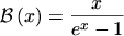$$\ensuremath{\mathcal{B} \left( x \right) }= \frac{x}{e^x - 1}$$ (3.53)

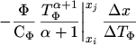
Beginning with

$$- \frac{\Phi}{\mathrm{C}_\Phi} = \frac{(\alpha + 1) \, \Delta T_\Phi}{\Delta x} \, \Bigl( \xi_j ... ...^{\alpha + 1}} {T_{\Phi \, j}^{\alpha + 1} - T_{\Phi \, i}^{\alpha + 1}} \Bigr)$$ (3.54)

$$= \frac{(\alpha + 1) \, \Delta T_\Phi}{\Delta x} \, \Bigl( \xi_j ... ... \xi_i \, \frac{1}{ (T_{\Phi \, j} / T_{\Phi \, i})^{\alpha + 1} - 1} \Bigr)\ ,$$ (3.55)

and using the abbreviations

$$(T_{\Phi \, i} / T_{\Phi \, j})^{\alpha + 1} = e^{(\alpha + 1) \, \ln(T_{\Phi \, i} / T_{\Phi \, j})} = e^{Y_\Phi} \ ,$$ (3.56)

$$Y_\Phi = (\alpha + 1) \, \ln(T_{\Phi \, i} / T_{\Phi \, j}) \ ,$$ (3.57)

$$\alpha + 1 = \frac{Y_\Phi}{\ln(T_{\Phi \, i} / T_{\Phi \, j})} \ ,$$ (3.58)

the flux equation can be written as

$$- \frac{\Phi}{\mathrm{C}_\Phi} = \frac{\Delta T_\Phi}{\Delta x} \, \frac{Y_\Phi}{\ln(T_{\Phi \, ... ...( \xi_j \, \frac{1}{1 - e^{Y_\Phi}} - \xi_i \, \frac{1}{e^{-Y_\Phi} - 1} \Bigr)$$ (3.59)

$$= \frac{\Delta T_\Phi}{\Delta x} \, \frac{1}{\ln(T_{\Phi \, j} / ... ...c{Y_\Phi}{e^{Y_\Phi} - 1} - \xi_i \, \frac{-Y_\Phi}{e^{-Y_\Phi} - 1} \Bigr) \ ,$$ (3.60)

or using the BERNOULLI function as

$$\Phi = - \frac{\mathrm{C}_\Phi}{\Delta x} \, \frac{\Delta T_\Phi} {\ln... ... \right) }- \xi_i \, \ensuremath{\mathcal{B} \left( -Y_\Phi \right) }\Bigr) \ ,$$ (3.61)

$$Y_\Phi = - \frac{\ln(T_{\Phi \, j} / T_{\Phi \, i})}{\Delta T_\Phi} \, \... ...ac{\mathrm{q}}{\mathrm{k}_\mathrm{B}} \, \Delta \psi + \Delta T_\Phi \Bigr) \ .$$ (3.62)

The concept of assuming a constant flux density was first presented by SCHARFETTER and GUMMEL in the appendix of [51, p.73]. The assumption of a linear variation of the generalized temperature $T_\Phi$ by eqn. (3.43) can be interpreted as a straightforward extension of the SCHARFETTER-GUMMEL scheme.

An advantage of using BERNOULLI functions in the flux equations is that $\ensuremath{\mathcal{B} \left( x \right) }$ is well defined at $x = 0$.

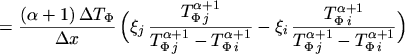
Inserting the abbreviations (3.38) to (3.40) used for $\xi$ and $T_\Phi$ yields the discretized flux equations

$$J_n = - \frac{\mathrm{C}_1}{\Delta x} \, \frac{\Delta T_n} {\ln(T_{n ... ... Y_1 \right) }- n_i \, \ensuremath{\mathcal{B} \left( - Y_1 \right) }\Bigr) \ ,$$ (3.63)

$$Y_1 = - \frac{\ln(T_{n \, j} / T_{n \, i})}{\Delta T_n} \, \Bigl( s_n... ...\frac{\mathrm{q}}{\mathrm{k}_\mathrm{B}} \, \Delta \psi + \Delta T_n \Bigr) \ ,$$ (3.64)

$$S_n = - \frac{\mathrm{C}_3}{\Delta x} \, \frac{\Delta (T_n \, \beta_n... ...- n_i \, T_{n \, i} \, \ensuremath{\mathcal{B} \left( - Y_3 \right) }\Bigr) \ ,$$ (3.65)

$$Y_3 = - \frac{\ln((T_{n \, j} \, \beta_{n \, j}) / (T_{n \, i} \, \be... ...{q}}{\mathrm{k}_\mathrm{B}} \, \Delta \psi + \Delta (T_n \, \beta_n) \Bigr) \ ,$$ (3.66)

$$K_n = - \frac{\mathrm{C}_5}{\Delta x} \, \frac{\Delta (T_n \, \beta_n... ...2 \, \beta_{n \, i} \, \ensuremath{\mathcal{B} \left( - Y_5 \right) }\Bigr) \ ,$$ (3.67)

$$Y_5 = - \frac{\ln((T_{n \, j} \, \beta_{n \, j}^2) / (T_{n \, i} \, \... ...}}{\mathrm{k}_\mathrm{B}} \, \Delta \psi + \Delta (T_n \, \beta_n^2) \Bigr) \ .$$ (3.68)

M. Gritsch: Numerical Modeling of Silicon-on-Insulator MOSFETs PDF