5.2.1 Anisotropic Distribution Function

In this section the flux equations of an energy transport model assuming an anisotropic distribution function will be derived. The balance equations are not affected by an anisotropic distribution function since the tensor quantities only appear in the odd moment equations (2.76) to (2.78).

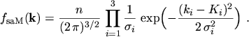
In order to allow for an anisotropic distribution function the starting point will be a MAXWELL distribution

$$f_\mathrm{M}(\ensuremath{\boldsymbol{\mathrm{k}}}) = \mathrm{A} \... ...}\, T_n} \Bigr) = \mathrm{A} \, \exp \Bigl( - \frac{k^2}{2 \, k_t^2} \Bigr) \ ,$$ (5.6)

where

$$k_t = \sqrt{\frac{m \, \mathrm{k}_\mathrm{B}\, T_n}{\hbar^2}}$$ (5.7)

is the standard deviation.

To get the value of the coefficient $\mathrm{A}$ the normalization

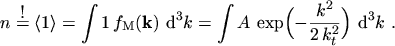$$n \stackrel{\textstyle !}{=} \ensuremath{\langle 1 \rangle}= \ens... ...exp \Bigl( - \frac{k^2}{2 \, k_t^2} \Bigr) \,\, \ensuremath{\mathrm{d}}^3 k}\ .$$ (5.8)

is used. By using spherical polar coordinates and the substitution $\ensuremath{\boldsymbol{\mathrm{k}}} = \ensuremath{\boldsymbol{\mathrm{k'}}} \, k_t$ the integral can be written as

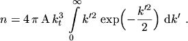$$n = 4 \, \pi \, \mathrm{A} \, k_t^3 \, \ensuremath{\int_0^{\infty} k'^2 \, \exp \Bigl( - \frac{k'^2}{2} \Bigr) \,\, \ensuremath{\mathrm{d}}k'}\ .$$ (5.9)

Setting $k' = \sqrt{2 \, t}$ gives

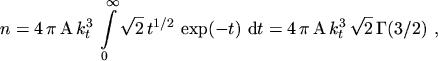$$n = 4 \, \pi \, \mathrm{A} \, k_t^3 \, \ensuremath{\int_0^{\infty... ...\mathrm{d}}t}= 4 \, \pi \, \mathrm{A} \, k_t^3 \, \sqrt{2} \, \Gamma(3 / 2) \ ,$$ (5.10)

where the GAMMA function has been used

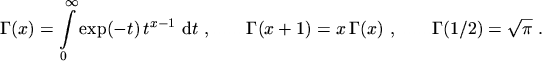$$\Gamma(x) = \ensuremath{\int_0^{\infty} \exp(-t) \, t^{x - 1} \,\... ...x \, \Gamma(x) \ , \textcolor{lightgrey}{.......}\Gamma(1 / 2) = \sqrt{\pi} \ .$$ (5.11)

The coefficient $\mathrm{A}$ and the distribution function is found to be

$$\mathrm{A} = \frac{n}{\bigl( \sqrt {2 \, \pi} \, k_t \bigr)^3} \ ,$$ (5.12)

$$f_\mathrm{M}(\ensuremath{\boldsymbol{\mathrm{k}}}) = \frac{n}{\bigl( \sqrt {2 \, \pi} \, k_t \bigr)^3} \, \exp \Bigl( - \frac{k^2}{2 \, k_t^2} \Bigr) \ .$$ (5.13)

An anisotropic MAXWELL distribution function is obtained by splitting the argument of the exponential function into three separate components

$$\frac{k^2}{k_t^2} = \frac{k_x^2 + k_y^2 + k_z^2}{k_t^2} \Rightarrow \frac{k_x^2}{\s... ...}_\mathrm{B}\, T_{ii}}{\hbar^2}} \ , \textcolor{lightgrey}{....}i = x, y, z \ ,$$ (5.14)

$$f_{\mathrm{aM}}(\ensuremath{\boldsymbol{\mathrm{k}}}) = n \, \prod_{i = 1}^3 \frac{1}{\sqrt{2 \, \pi}} \, \frac{1}{\sigma_i} \, \exp \Bigl( - \frac{k_i^2}{2 \, \sigma_i^2} \Bigr) \ .$$ (5.15)

Since the odd moments of this distribution function are zero, current flow would not be possible. To allow for current flow, the distribution function is shifted

$$f_\mathrm{saM}(\ensuremath{\boldsymbol{\mathrm{k}}}) = \frac{n}{(... ...{1}{\sigma_i} \, \exp \Bigl( - \frac{(k_i - K_i)^2}{2 \, \sigma_i^2} \Bigr) \ .$$ (5.16)

Again, the diffusion approximation is applied which assumes that the displacement is small, $\frac{K_i}{\sigma_i} \ll 1$,

$$f_\mathrm{saM} \Bigl( \frac{k_x - K_x}{\sigma_x}, \frac{k_y - K_y}{\sigma_y}, \frac{k_z - K_z}{\sigma_z} \Bigr) \approx$$

$$\approx f_{\mathrm{aM}}\Bigl( \frac{k_x}{\sigma_x}, \frac{k_y}{\s... ...{\partial f_{\mathrm{aM}}}{\partial (k_z / \sigma_z)} \, \frac{K_z}{\sigma_z} =$$ (5.17)

$$= f_\mathrm{aM}(\ensuremath{\boldsymbol{\mathrm{k}}}) \, \Bigl( 1... ...x^2} + \frac{k_y \, K_y}{\sigma_y^2} + \frac{k_z \, K_z}{\sigma_z^2} \Bigr) \ .$$

The symmetric and the anti-symmetric part are found to be

$$f_\mathrm{S}(\ensuremath{\boldsymbol{\mathrm{k}}}) = f_\mathrm{aM}(\ensuremath{\boldsymbol{\mathrm{k}}}) \ ,$$ (5.18)

$$f_\mathrm{A}(\ensuremath{\boldsymbol{\mathrm{k}}}) = f_\mathrm{S}(\ensuremath{\boldsymbol{\mathrm{k}}}) \, \sum_{i=1}^3 \frac{k_i \, K_i}{\sigma_i^2} \ .$$ (5.19)

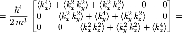
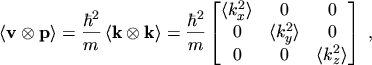
The equations for the current density and the energy flux density are obtained by calculating the statistical averages of the tensors occurring in eqns. (2.76) and (2.77)

$$\ensuremath{\langle \mathcal{E} \rangle}= \frac{\hbar^2}{2 \, m} ... ...ensuremath{\langle k_y^2 \rangle}+ \ensuremath{\langle k_z^2 \rangle}\bigr) \ ,$$ (5.20)

$$\ensuremath{\langle \ensuremath{\boldsymbol{\mathrm{v}}} \ensurem... ..._y^2 \rangle}& 0 \\ 0 & 0 & \ensuremath{\langle k_z^2 \rangle}\end{bmatrix} \ ,$$ (5.21)

$$\ensuremath{\langle \ensuremath{\boldsymbol{\mathrm{v}}} \ensuremath{\otimes}\ensuremath{\boldsymbol{\mathrm{v}}} \, \mathcal{E} \rangle} = \ensuremath{\langle \frac{\hbar \, \ensuremath{\boldsymbol{\mat... ...emath{\boldsymbol{\mathrm{k}}} \, \bigl( k_x^2 + k_y^2 + k_z^2 \bigr) \rangle}=$$

$$= \frac{\hbar^4}{2 \, m^3} \, \ensuremath{\langle \begin{bmatrix}... ...\\ 0 & 0 & k_z^2 \end{bmatrix} \, \bigl( k_x^2 + k_y^2 + k_z^2 \bigr) \rangle}=$$ (5.22)

$$= \frac{\hbar^4}{2 \, m^3} \, \begin{bmatrix}\ensuremath{\langle ... ...k_y^2 \, k_z^2 \rangle}+ \ensuremath{\langle k_z^4 \rangle}\\ \end{bmatrix} \ .$$

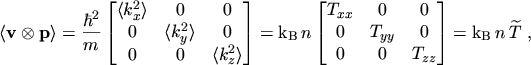
The elements outside the trace are zero due to the symmetry properties of $f_\mathrm{S}$, introduced by the diffusion approximation. The statistical averages present in eqns. (5.20) to (5.23) all have one of the forms $\ensuremath{\langle k_x^2 \rangle}$, $\ensuremath{\langle k_x^4 \rangle}$, or $\ensuremath{\langle k_x^2 \, k_y^2 \rangle}$, and will be integrated in the following.

$$\ensuremath{\langle k_x^2 \rangle} = \ensuremath{\iiint\limits_{-\infty}^{\ \ \ \infty} k_x^2 \, f_\... ...\Bigr( - \frac{k_x^2}{2 \, \sigma_x^2} \Bigr) \,\, \ensuremath{\mathrm{d}}k_x}=$$

$$= \frac{\sigma_x^2}{\sqrt{\pi}} \, 2 \, n \ensuremath{\int_0^{\in... ... n \, \sigma_x^2 = \frac{m \, \mathrm{k}_\mathrm{B}\, n \, T_{xx}}{\hbar^2} \ ,$$ (5.23)

$$\ensuremath{\langle k_x^4 \rangle} = \ensuremath{\iiint\limits_{-\infty}^{\ \ \ \infty} k_x^4 \, f_\... ...\Bigr( - \frac{k_x^2}{2 \, \sigma_x^2} \Bigr) \,\, \ensuremath{\mathrm{d}}k_x}=$$

$$= \frac{\sigma_x^4}{\sqrt{\pi}} \, 4 \, n \ensuremath{\int_0^{\in... ..._x^4 = \frac{3 \, m^2 \, \mathrm{k}_\mathrm{B}^2 \, n \, T_{xx}^2}{\hbar^4} \ ,$$ (5.24)

$$\ensuremath{\langle k_x^2 \, k_y^2 \rangle} = \frac{n}{2 \, \pi} \, \ensuremath{\int_{-\infty}^{\infty} k_x^2... ...\Bigr( - \frac{k_y^2}{2 \, \sigma_y^2} \Bigr) \,\, \ensuremath{\mathrm{d}}k_y}=$$

$$= n \, \sigma_x^2 \, \sigma_y^2 = \frac{m^2 \, \mathrm{k}_\mathrm{B}^2 \, n \, T_{xx} \, T_{yy}}{\hbar^4} \ .$$ (5.25)

Inserting these results into eqns. (5.20) to (5.23) finally yields

$$\ensuremath{\langle \mathcal{E} \rangle}= \frac{\hbar^2}{2 \, m} ... ... \stackrel{\textstyle !}{=} \frac{3}{2} \, \mathrm{k}_\mathrm{B}\, n \, T_n \ ,$$ (5.26)

which reflects eqn. (5.5),

$$\ensuremath{\langle \ensuremath{\boldsymbol{\mathrm{v}}} \ensurem... ...{zz} \end{bmatrix} = \mathrm{k}_\mathrm{B}\, n \, \ensuremath{\widetilde{T}}\ ,$$ (5.27)

and

$$\ensuremath{\langle \ensuremath{\boldsymbol{\mathrm{v}}} \ensuremath{\otimes}\ensuremath{\boldsymbol{\mathrm{v}}} \, \mathcal{E} \rangle} = \frac{\hbar^4}{2 \, m^3} \, \begin{bmatrix}\ensuremath{\langle ... ...e k_y^2 \, k_z^2 \rangle}+ \ensuremath{\langle k_z^4 \rangle}\\ \end{bmatrix} =$$

$$= \frac{\mathrm{k}_\mathrm{B}^2 \, n}{2 \, m} \, \begin{bmatrix}3... ...{.......}T_{xx} \, T_{zz} + T_{yy} \, T_{zz} + 3 \, T_{zz}^2 \\ \end{bmatrix} =$$

$$= \frac{\mathrm{k}_\mathrm{B}^2 \, n}{2 \, m} \, \begin{bmatrix}T... .........}T_{zz} \, \bigl( T_{xx} + T_{yy} + 3 \, T_{zz} \bigr) \\ \end{bmatrix} =$$ (5.28)

$$= \frac{\mathrm{k}_\mathrm{B}^2 \, n}{2 \, m} \, \begin{bmatrix}T... ...grey}{.......}T_{zz} \, \bigl( 2 \, T_{zz} + 3 \, T_n \bigr) \\ \end{bmatrix} =$$

$$= \frac{\mathrm{k}_\mathrm{B}^2 \, n}{2 \, m} \, \begin{bmatrix}T... ...n & 0 & 0 \\ 0 & 3 \, T_n & 0 \\ 0 & 0 & 3 \, T_n \end{bmatrix} \end{bmatrix} =$$

$$= \frac{\mathrm{k}_\mathrm{B}^2 \, n}{2 \, m} \, \bigl( 2 \, \ens... ..., T_n \, \ensuremath{\widetilde{\delta}}\bigr) \, \ensuremath{\widetilde{T}}\ .$$

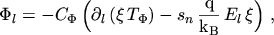
The flux equations of the anisotropic energy transport model thus become

$$\ensuremath{\boldsymbol{\mathrm{J}}}_n = - \frac{\mathrm{q}}{m} \... ...e{T}} \bigr)}+ \mathrm{q}\, \ensuremath{\boldsymbol{\mathrm{E}}}\, n \Bigr) \ ,$$ (5.29)

$$\ensuremath{\boldsymbol{\mathrm{S}}}_n = \ensuremath{\langle \ensuremath{\boldsymbol{\mathrm{v}}} \, \mathcal{E} \rangle} = - \tau_S \, \Bigl( \ensuremath{\ensuremath{\ensuremath{\boldsym... ...1}{m} \, \mathrm{k}_\mathrm{B}\, n \, \ensuremath{\widetilde{T}}\Bigr) \Bigr) =$$

$$= - \frac{\tau_S \, \mathrm{k}_\mathrm{B}^2}{2 \, m} \, \Bigl( \e... ...nsuremath{\widetilde{\delta}}+ 2 \, \ensuremath{\widetilde{T}}\Bigr) \Bigr) \ ,$$ (5.30)

and their one-dimensional projection onto an arbitrary direction $\ensuremath{\boldsymbol{\mathrm{e}}}_l$ reads

$$J_{n, \, l} = \underbrace{\frac{\mathrm{q}\, \tau_m}{m}}_{\textstyle \mu_n} \... ...( \mathrm{k}_\mathrm{B}\, n \, T_{ll} \bigr)}+ \mathrm{q}\, E_l \, n \Bigr) \ ,$$ (5.31)

$$S_{n, \, l} = - \underbrace{\frac{\mathrm{q}\, \tau_m}{m}}_{\textstyle \mu_n}... ...}}{\mathrm{k}_\mathrm{B}} \, n \, E_l \, \bigl( 3 \, T_n + 2 \, T_{ll} \bigr) =$$

$$= - \frac{5}{2} \, \mu_n \, \frac{\tau_S}{\tau_m} \, \frac{\mathr... ...athrm{k}_\mathrm{B}} \, E_l \, n \, \frac{3 \, T_n + 2 \, T_{ll}}{5} \Bigr) \ ,$$ (5.32)

In terms of the general flux equation (3.41)

$$\Phi_l = - C_\Phi \, \Bigl( \ensuremath{\partial_{l} \, (\xi \, T_\Phi)}- s_n \, \frac{\mathrm{q}}{\mathrm{k}_\mathrm{B}} \, E_l \, \xi \Bigr) \ ,$$ (5.33)

the quantities $\mathrm{C}_\Phi$, $\xi$, and $T_\Phi$ read

$$\ensuremath{\boldsymbol{\mathrm{J}}}_n : \textcolor{lightgrey}{.......}\mathrm{C}_\Phi = s_n \, \mathrm{k}_\mathrm{B}\, \mu_n \ , \textcolor{lightgrey}{.......}\xi = n \ , \textcolor{lightgrey}{.......}T_\Phi = T_{ll} \ ,$$ (5.34)

$$\ensuremath{\boldsymbol{\mathrm{S}}}_n : \textcolor{lightgrey}{.......}\mathrm{C}_\Phi = \frac{5}{2} \, \frac{\mathrm{k}_\mathrm{B}^2}{\mathrm{q}} \, \frac{\tau_S}{\tau_m} \, \mu_n \ , \textcolor{lightgrey}{.......}\xi = n \, \frac{3 \, T_n + 2 \, T_{ll}}{5} \ , \textcolor{lightgrey}{.......}T_\Phi = T_{ll} \ .$$ (5.35)

Note that the discretization eqn. (3.61) can be used without modification.

M. Gritsch: Numerical Modeling of Silicon-on-Insulator MOSFETs PDF