6.2.3 Inhomogeneous Case

In this section heuristic models for $\beta _n$ will be presented, which have been fitted to Monte Carlo results of $n^+$-$n$-$n^+$ test structures.

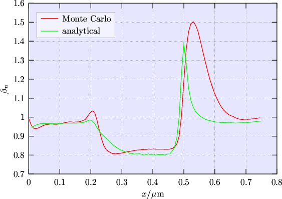
The points B and E in Fig. 5.5 can be distinguished by taking, for example, the gradient of the carrier temperature into account. To capture both the $\beta_n < 1$ and $\beta_n > 1$ region (Fig. 6.4), such a dependence on the gradient of the carrier temperature is introduced:

Figure 6.4: Monte Carlo simulation of an $n^+$-$n$-$n^+$ structure showing the normalized moment of fourth order $\beta _{n,\textrm {MC}}$ compared to the analytical $\beta _{n,1}$.

$$\beta_{n, 1} = \Bigl( 1 - \frac{\ensuremath{\ensuremath{\ensurema... ...or{lightgrey}{.......}U_T = \frac{\mathrm{k}_\mathrm{B}}{\mathrm{q}} \, T_n \ .$$ (6.12)

To account for the non-parabolic band structure used in the Monte Carlo simulation a non-parabolicity factor due to BORDELON [73] [74] is included

$$\beta_\mathrm{Bord}(T_n) = \frac{3}{5} \, H(T_n) \, \Bigl( 1 + \frac{2}{3} \, H(T_n) \Bigr) \ ,$$ (6.13)

$$H(T_n) = \frac{1 + \alpha \, \frac{3}{2} \, \frac{\mathrm{k}_\mathrm{B}\... ...athrm{q}}} , \textcolor{lightgrey}{.......}\alpha = 0.5 \, \mathrm{eV}^{-1} \ .$$ (6.14)

The model (6.12) reproduces the peak of $\beta _n$ in the region where the hot carriers from the channel mix with the cold ones in the drain (Fig. 6.4). In this way, the hysteresis of $\beta _n$ shown in Fig. 6.5 can also be reproduced at least qualitatively.

Figure 6.5: Monte Carlo simulation of an $n^+$-$n$-$n^+$ structure showing the hysteresis of the normalized moment of fourth order $\beta _{n,\textrm {MC}}$ compared to the analytical $\beta _{n,1}$.

However, the model eqn. (6.12) leads to severe stability problems with the numerical iteration. Furthermore it turned out that the reproduction of the peak is not essential for solving the problem related to SOI simulations since the important point is to allow for a reduced $\beta _n$ along the channel--especially in the pinch-off region.

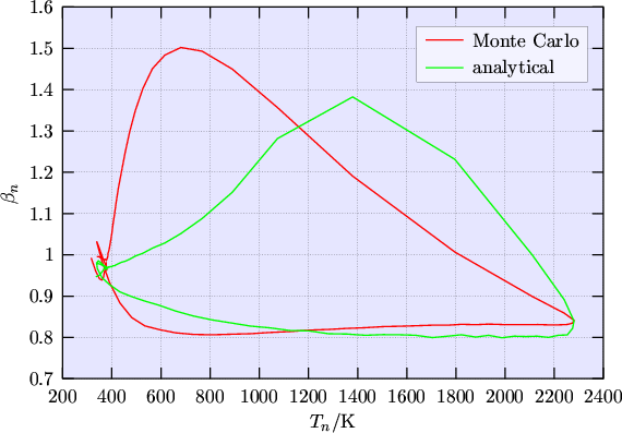
In most of the channel region the high energy tail is less populated than that of a MAXWELLian distribution which means that $\beta_n < 1$ (Fig. 6.6). It is believed that proper modeling of the $\beta_n < 1$ region is very important for the SOI problem described in Chapter 4, because the smaller amount of carriers in the high energy tail will give reduced hot carrier diffusion into the floating body.

Figure 6.6: Comparison of the non-MAXWELLian parameter obtained by Monte Carlo simulations and the empirical model $\beta _{n,2}$.

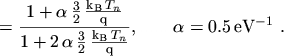
To avoid numerical stability problems a model for $\beta _n$ as a function of $T_n$ only has been developed

$$\beta_{n, 2} = \beta_0 + \bigl( 1 - \beta_0 \bigr) \, \exp \Bigl( - \Bigl( \frac{T_n - T_\mathrm{L}}{\mathrm{T_{ref, \beta}}} \Bigr)^2 \Bigr) \ ,$$ (6.15)

which neglects the peak in the drain region (mixing of hot and cold distributions). Parameters are only weakly dependent on doping and applied voltage which can be seen by comparing Fig. 6.4 and Fig. 6.6 which were obtained by using two different devices.

M. Gritsch: Numerical Modeling of Silicon-on-Insulator MOSFETs PDF