7.1 Übliche Randbedingungen für das magnetische Vektorpotenzial

Abbildung 7.1: Simulationsbereich und Ränder bei der Berechnung des magnetischen Vektorpotenzials: Die beiden stromführenden Segmente ${\cal{V}}_a$ und ${\cal{V}}_b$ erfüllen unten angeführte Randbedingungen. Da keine magnetischen Materialien behandelt werden, sind die Stetigkeitsbedingungen $\mathchoice{\mbox{\boldmath$\displaystyle n$}} {\mbox{\boldmath$\textstyle n$}... ...} {\mbox{\boldmath$\scriptstyle H$}} {\mbox{\boldmath$\scriptscriptstyle H$}}_2$ (vergleiche (7.5)) und $\mathchoice{\mbox{\boldmath$\displaystyle n$}} {\mbox{\boldmath$\textstyle n$}... ...} {\mbox{\boldmath$\scriptstyle H$}} {\mbox{\boldmath$\scriptscriptstyle H$}}_2$ (Flächenstromdichte auf $\Gamma_H$ gleich Null) an den Grenzflächen implizit erfüllt.

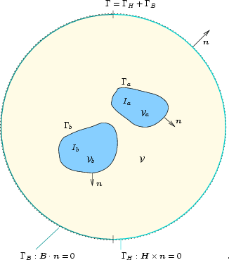
Die Randbedingungen für magnetische Felder sind Vorgaben für Feldstärke bzw. Flußdichte. Um die Eindeutigkeit des Vektorpotenzials sicherzustellen, genügen die Vorgaben allerdings nicht. Auf dem Rand $\Gamma$ (s. Abb. 7.1) muss zusätzlich immer die Tangential- oder die Normalkomponente des Vektorpotenzials festgelegt werden [145]. Um eine eindeutige Lösung zu erhalten, muss außerdem zumindest ein (beliebiger) Knoten eine Dirichlet-Bedingung erfüllen, indem der diesem Knoten zugeordnete Funktionswert auf einen beliebigem Wert, praktischerweise Null, gesetzt wird.

Die Oberfläche $\Gamma$ ist in zwei Teile geteilt, da besonders zwei Randbedingungen von praktischer Bedeutung sind: Auf $\Gamma _B$ ist die Normalkomponente der Flußdichte vorgeschrieben, während auf $\Gamma _H$ die Tangentialkomponente der magnetischen Feldstärke gegeben ist. Was diese Vorgaben, (7.5) und (7.6), für das magnetische Vektorpotenzial bedeuten, wird nun ausgeführt:

$$\mathchoice{\mbox{\boldmath$\displaystyle n$}} {\mbox{\boldmath$\... ...$}} {\mbox{\boldmath$\scriptstyle B$}} {\mbox{\boldmath$\scriptscriptstyle B$}} =0\quad\rm {auf}\quad\Gamma _B,$$ (7.5)

$$\mathchoice{\mbox{\boldmath$\displaystyle n$}} {\mbox{\boldmath$\... ...$}} {\mbox{\boldmath$\scriptstyle H$}} {\mbox{\boldmath$\scriptscriptstyle H$}} =\mathchoice{\mbox{\boldmath$\displaystyle 0$}} {\mbox{\boldmath$... ...tyle 0$}} {\mbox{\boldmath$\scriptscriptstyle 0$}}\quad\rm {auf}\quad\Gamma _H.$$ (7.6)

Diese beiden Randbedingungen werden mit dem magnetischen Vektorpotenzial folgendermaßen formuliert

$$\mathchoice{\mbox{\boldmath$\displaystyle n$}} {\mbox{\boldmath$\... ...$}} {\mbox{\boldmath$\scriptstyle A$}} {\mbox{\boldmath$\scriptscriptstyle A$}} =0\quad \rm {auf} \quad\Gamma _B,$$ (7.7)

$$\frac{1}{\protect{\mbox{{\usefont{U}{eur}{m}{n}\char22}}}}\nabla\... ...$}} {\mbox{\boldmath$\scriptstyle n$}} {\mbox{\boldmath$\scriptscriptstyle n$}} =\mathchoice{\mbox{\boldmath$\displaystyle 0$}} {\mbox{\boldmath$... ...yle 0$}} {\mbox{\boldmath$\scriptscriptstyle 0$}}\quad \rm {auf}\quad\Gamma _H.$$ (7.8)

Gleichung (7.7) kann nach [115] ersetzt werden durch

$$\mathchoice{\mbox{\boldmath$\displaystyle n$}} {\mbox{\boldmath$\... ...$}} {\mbox{\boldmath$\scriptstyle A$}} {\mbox{\boldmath$\scriptscriptstyle A$}} =\mathchoice{\mbox{\boldmath$\displaystyle 0$}} {\mbox{\boldmath$... ...tyle 0$}} {\mbox{\boldmath$\scriptscriptstyle 0$}}\quad\rm {auf}\quad\Gamma _B,$$ (7.9)

und stellt somit auch die Eindeutigkeit von $\mathchoice{\mbox{\boldmath $\displaystyle A$}} {\mbox{\boldmath $\textstyle A$}} {\mbox{\boldmath $\scriptstyle A$}} {\mbox{\boldmath $\scriptscriptstyle A$}}$ sicher. Diese Dirichlet-Randbedingung ist durch die Vorgabe der Tangentialkomponente auf der Oberfläche $\Gamma _B$ gekennzeichnet. Homogene Dirichlet-Randbedingungen ( $\mathchoice{\mbox{\boldmath $\displaystyle A$}} {\mbox{\boldmath $\textstyle A... ...mbox{\boldmath $\scriptstyle A$}} {\mbox{\boldmath $\scriptscriptstyle A$}}_t=0$), entsprechend (7.9), bedeuten bei unendlich langer, gerader Grenze $\Gamma _B$ (s. Abb. 7.2) eine antisymmetrische Spiegelung von Quellenstromdichten. Es dürfen somit in der Symmetrieebene nur Normalkomponenten von Quellenströmen auftreten, das resultierende Magnetfeld verläuft entsprechend (7.5) tangential.

Abbildung 7.2: Antisymmetrische Spiegelung von Quellen durch homogene Dirichlet-Randbedingungen

Eine ideal leitfähige (supraleitende) Oberfläche kann durch eine homogene Dirichlet-Randbedingung für das Vektorpotenzial $\mathchoice{\mbox{\boldmath $\displaystyle A$}} {\mbox{\boldmath $\textstyle A$}} {\mbox{\boldmath $\scriptstyle A$}} {\mbox{\boldmath $\scriptscriptstyle A$}}$ repräsentiert werden. Wenn ein magnetisches Feld außerhalb des Leiters existiert, werden Oberflächenströme derart induziert, dass das Innere des Leiters feldfrei bleibt.

Homogene Neumannsche Randbedingungen sind durch (7.8) gegeben und haben bei unendlich langer, gerader Grenze (siehe Abb. 7.3) eine symmetrische Spiegelung der Quellenstromdichten zur Folge. In der Symmetrieebene dürfen somit nur tangentiale Quellenströme fließen, das Magnetfeld verläuft senkrecht zur Begrenzungsfläche. Um das Vektorpotenzial eindeutig zu machen, ist es notwendig, dessen Divergenz und auf der Oberfläche $\Gamma$ des Bereichs $\cal V$, entweder seine Normal- oder Tangentialkomponente zu definieren [115]. Da die Tangentialkomponente von $\mathchoice{\mbox{\boldmath $\displaystyle A$}} {\mbox{\boldmath $\textstyle A$}} {\mbox{\boldmath $\scriptstyle A$}} {\mbox{\boldmath $\scriptscriptstyle A$}}$ auf der Oberfläche $\Gamma _B$ schon vorgegeben wurde, ist es naheliegend seine Normalkomponente auf $\Gamma _H$ festzulegen. Man erreicht dies durch die Einführung der zusätzlichen Randbedingung [146]

$$\mathchoice{\mbox{\boldmath$\displaystyle n$}} {\mbox{\boldmath$\... ...$}} {\mbox{\boldmath$\scriptstyle A$}} {\mbox{\boldmath$\scriptscriptstyle A$}} =0\quad \rm {auf}\quad \Gamma _H.$$ (7.10)

Abbildung 7.3: Symmetrische Spiegelung von Quellen durch homogeneNeumannsche Randbedingungen

Zusammenfassend werden noch einmal mögliche Bedingungen angeführt, die ein eindeutiges Vektorpotenzial sicherstellen [115]:

$$\nabla\!\times\!\mathchoice{\mbox{\boldmath$\displaystyle A$}} {\... ...$}} {\mbox{\boldmath$\scriptstyle A$}} {\mbox{\boldmath$\scriptscriptstyle A$}} =\mathchoice{\mbox{\boldmath$\displaystyle B$}} {\mbox{\boldmath$... ...tstyle B$}} {\mbox{\boldmath$\scriptscriptstyle B$}}\quad\mathrm{in}\,{\cal V},$$

$$\nabla\!\cdot\!\mathchoice{\mbox{\boldmath$\displaystyle A$}} {\m... ...$}} {\mbox{\boldmath$\scriptstyle A$}} {\mbox{\boldmath$\scriptscriptstyle A$}} =0\quad\mathrm{in}\,{\cal V},$$

$$\mathchoice{\mbox{\boldmath$\displaystyle n$}} {\mbox{\boldmath$\... ...$}} {\mbox{\boldmath$\scriptstyle A$}} {\mbox{\boldmath$\scriptscriptstyle A$}} =\mathchoice{\mbox{\boldmath$\displaystyle 0$}} {\mbox{\boldmath$... ...tyle 0$}} {\mbox{\boldmath$\scriptscriptstyle 0$}}\quad\mathrm{auf}\,\Gamma _B,$$

$$\mathchoice{\mbox{\boldmath$\displaystyle n$}} {\mbox{\boldmath$\... ...$}} {\mbox{\boldmath$\scriptstyle A$}} {\mbox{\boldmath$\scriptscriptstyle A$}} =0\quad\mathrm{auf}\,\Gamma _H.$$

Die hier angegebenen Randbedingungen führen zu einer Verkoppelung der drei Gleichungssysteme für jede Komponente von $\mathchoice{\mbox{\boldmath $\displaystyle A$}} {\mbox{\boldmath $\textstyle A$}} {\mbox{\boldmath $\scriptstyle A$}} {\mbox{\boldmath $\scriptscriptstyle A$}}$. Die verfolgte Strategie bevorzugt deshalb als Randbedingung am fernen Rand $\mathchoice{\mbox{\boldmath $\displaystyle A$}} {\mbox{\boldmath $\textstyle A... ...} {\mbox{\boldmath $\scriptstyle 0$}} {\mbox{\boldmath $\scriptscriptstyle 0$}}$ vorzugeben, da dies zu drei entkoppelten Poisson-Gleichungen führt. Das Simulationsgebiet muss ohnehin groß genug sein, damit das Feld nicht verzerrt wird.

Die Ausnutzung der Symmetrie durch die entsprechenden homogenen Randbedingungen kann den Berechnungsaufwand eines Problems wesentlich reduzieren. Sind jedoch Randbedingungen vorzugeben, wo Spiegelungen unerwünscht sind, so muss deren Einfluss gering gehalten werden. Deshalb wird der Rand weit genug vom eigentlich interessierenden Feldgebiet weggerückt [147].