. In [61] they presented a correction scheme for (4.3),
which is based on the determination of the accumulated degradation due to stress
after the delay time
. In [61] they presented a correction scheme for (4.3),
which is based on the determination of the accumulated degradation due to stress
after the delay time  as
as
Grasser et al. refined the approach of [6, 88] to obtain universality irrespective of
the amount of . In [61] they presented a correction scheme for (4.3),
which is based on the determination of the accumulated degradation due to stress
after the delay time as
 | (4.4) |
Here,  splits up into
  , the recoverable amount of degradation monitored
at
, the recoverable amount of degradation monitored
at  , and a permanent components
  which is regarded as independent of
 . In [29],
  was supposed to follow a power-law of the form
 . In order to characterize the temperature and bias dependence of
the components of (4.4), plasma-nitrided-oxide (PNO) devices with an
effective oxide thickness (EOT) of
. In order to characterize the temperature and bias dependence of
the components of (4.4), plasma-nitrided-oxide (PNO) devices with an
effective oxide thickness (EOT) of  and
and  were characterized.
Therefore the OTF-method [17] and the fast-
were characterized.
Therefore the OTF-method [17] and the fast- -method developed by
[11] were used. The latter method is embedded into an eMSM-sequence
which is carried out with
-method developed by
[11] were used. The latter method is embedded into an eMSM-sequence
which is carried out with  stress/relaxation-subsequences, already
described in Chapter 2.1. A typical eMSM-measurement is shown in
Fig. 4.3.
stress/relaxation-subsequences, already
described in Chapter 2.1. A typical eMSM-measurement is shown in
Fig. 4.3.
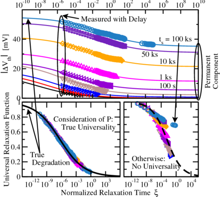
 is matched on the relaxation model (4.5)
with
is matched on the relaxation model (4.5)
with  parameters. It yields perfect universality over more than
  decades in time (lines). Bottom Left: After subtracting the single
  of
each relaxation sequence (marked above), all data can be fit to a single line.
The universality of the relaxing component
of
each relaxation sequence (marked above), all data can be fit to a single line.
The universality of the relaxing component  is clearly visible. Bottom
Right: Without considering
is clearly visible. Bottom
Right: Without considering  , data at large stress times does not conform
to the universality.
, data at large stress times does not conform
to the universality.
For the extraction of  and
and  , the yet unknown permanent contributions
of the single relaxation phases
, the yet unknown permanent contributions
of the single relaxation phases  have to be determined simultaneously. The
remaining non-permanent parts of the relaxation sequences are then fit to the
universal relaxation law (4.2). Altogether this yields a relaxation model with
have to be determined simultaneously. The
remaining non-permanent parts of the relaxation sequences are then fit to the
universal relaxation law (4.2). Altogether this yields a relaxation model with
 parameters
 and
and  are fit parameters for the universal recoverable component
 , and the
  with
with  denote the
  relaxation sequences which
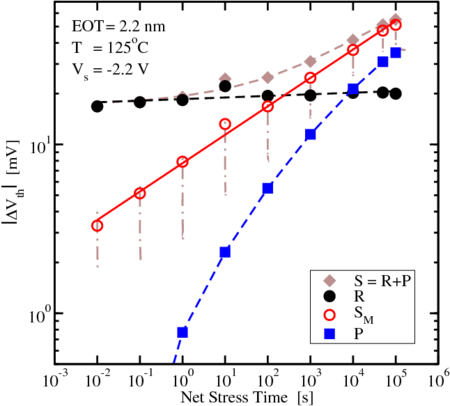
have to be optimized. The results of the optimization loop are then illustrated in
Fig. 4.4, clearly showing the existence of a permanent (or slowly relaxing)
component [30], when the recovery levels off. In contrast to
relaxation sequences which
have to be optimized. The results of the optimization loop are then illustrated in
Fig. 4.4, clearly showing the existence of a permanent (or slowly relaxing)
component [30], when the recovery levels off. In contrast to  , which can be
fitted by a power-law or
, which can be
fitted by a power-law or  ,
,  behaves like a power-law for
shorter stress times only. It clearly shows signs of saturation at longer stress
times, which is fundamental for lifetime extrapolation. Without considering such
a permanent component, universality is not given, like shown in Fig. 4.3 (bottom
left).
behaves like a power-law for
shorter stress times only. It clearly shows signs of saturation at longer stress
times, which is fundamental for lifetime extrapolation. Without considering such
a permanent component, universality is not given, like shown in Fig. 4.3 (bottom
left).
 and
the extracted recoverable and permanent components
and
the extracted recoverable and permanent components  and
and  .
By back-extrapolating
.
By back-extrapolating  the “real” total degradation
 is obtained, consisting of
  (compare to the true
degradation depicted left). The relaxation data in-between the stress
sequences is indicated by dash-dotted lines on a relative time scale
(compare to the true
degradation depicted left). The relaxation data in-between the stress
sequences is indicated by dash-dotted lines on a relative time scale
 . The recoverable component
  can be well fit by either a
power-law or
can be well fit by either a
power-law or  (used in the following) while
  closely
follows
closely
follows  after [6].
Moreover, it is of utmost importance to study wide relaxation periods, as the
data gained that way yields a much more reliable basis for modeling, compared
to other measurements done on commercial equipment: While Alam et al.
covered about  decades in time [85, 49], the widest recovery behavior observed
with commercial equipment so far accounted for
decades in time [85, 49], the widest recovery behavior observed
with commercial equipment so far accounted for  decades time [6, 66, 40].
Using their dedicated equipment Reisinger et al. [11] were able to measure BTI
relaxation periods of
decades time [6, 66, 40].
Using their dedicated equipment Reisinger et al. [11] were able to measure BTI
relaxation periods of  to
to  decades in time with the shortest available delay
time of
decades in time with the shortest available delay
time of  , cf. Fig. 4.3.
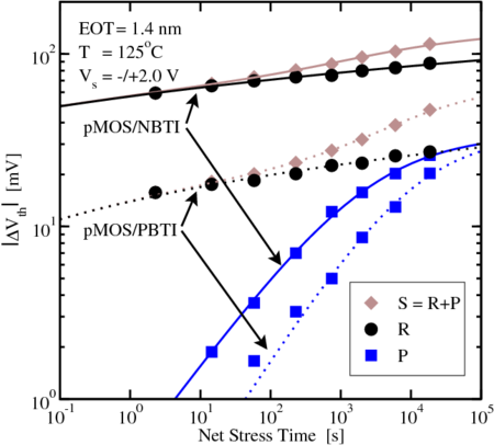
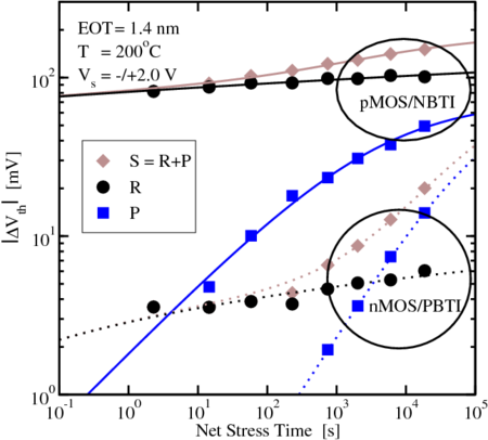
Applying the universality on various pMOS/nMOS-NBTI/PBTI-combinations yields different quantitative, but all in all consistent results. Surprisingly, this also applies to the negative shift of the threshold voltage they all have in common, for details refer to Fig. 4.5 and Fig. 4.6.
 compared to the devices of Fig. 4.3 and Fig. 4.4
with
compared to the devices of Fig. 4.3 and Fig. 4.4
with  , a considerably larger
  but a comparable
  component.
The recoverable component during PBTI stress is qualitatively the same but
shifted by a factor of
component.
The recoverable component during PBTI stress is qualitatively the same but
shifted by a factor of  to smaller values, while the permanent component
is quite similar compared to NBTI.
to smaller values, while the permanent component
is quite similar compared to NBTI.
 compared to the devices of Fig. 4.3
and Fig. 4.4 with
compared to the devices of Fig. 4.3
and Fig. 4.4 with  , a considerably larger
  but a comparable
 component. Comparison of pMOS/NBTI and nMOS/PBTI stress. The
recoverable component of the nMOS is very small (
component. Comparison of pMOS/NBTI and nMOS/PBTI stress. The
recoverable component of the nMOS is very small ( ). Hence, the
degradation is dominated by
). Hence, the
degradation is dominated by  from an early stage when comparing it to
pMOS.
from an early stage when comparing it to
pMOS.