7.3 Extraction Routine
The determination of the curvature following bias temperature stress is displayed
in Fig. 7.5. First, each relaxation of  is referred to its initial
  and is
plotted as
and is
plotted as  as a function of
  . The first decades as well
as the last decade in time are used to fit the experimental data with
a logarithm of the form
. The first decades as well
as the last decade in time are used to fit the experimental data with
a logarithm of the form  , giving the initial and long term
recovery behavior. Eventually, the intersection of the two fits results in the
“kink points”
, giving the initial and long term
recovery behavior. Eventually, the intersection of the two fits results in the
“kink points”  and
and  . While
  is used to describe the initial
recovery phase generally observed after PBTI,
is used to describe the initial
recovery phase generally observed after PBTI,  is used for the long
term recovery as observed after NBTI. These two cases are depicted in
the right of Fig. 7.4. However, the kink-point-method does not work
properly with too similar logarithmic prefactors
is used for the long
term recovery as observed after NBTI. These two cases are depicted in
the right of Fig. 7.4. However, the kink-point-method does not work
properly with too similar logarithmic prefactors  and
and  due to glancing
intersection, compare
due to glancing
intersection, compare  and
and  in Fig. 7.5. For
the already discussed complete recovery trace with its S-shape, the first
and second fit become nearly parallel resulting in an undetermined kink
point.
in Fig. 7.5. For
the already discussed complete recovery trace with its S-shape, the first
and second fit become nearly parallel resulting in an undetermined kink
point.
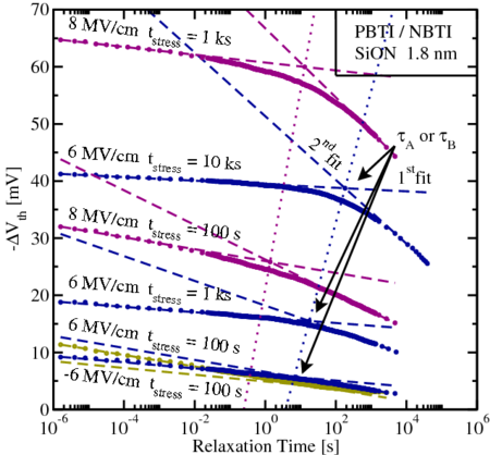
 or
or  at the extrapolated
intersection of the fits can be obtained, which characterizes the curvature.
Comparing kink points of the same electric field and oxide thickness for
different stress times (connected by dotted lines) shows that this curvature
is stronger at longer stress times and delayed with time.
at the extrapolated
intersection of the fits can be obtained, which characterizes the curvature.
Comparing kink points of the same electric field and oxide thickness for
different stress times (connected by dotted lines) shows that this curvature
is stronger at longer stress times and delayed with time.