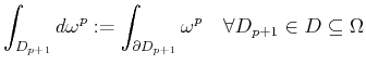
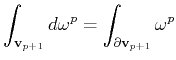
Several issues related to the differential formulation of the Maxwell equations were presented in Section 1.2. Finally, this section introduces a concise way of formulating physical problems regarding the fiber bundle and algebraic topology concepts. Starting with the integral formulation and partially reinserting the geometrical objects expressed in vector calculus notation, but omitting the orientation reads:
 |
(1.51) |
 |
(1.52) |
A better-suited representation, which directly references the oriented
geometric object a quantity is assigned to, is given with the
formalism of ordinary and twisted differential forms which can be seen
as the continuous counterpart of cochains, as introduced in Section
1.4.
For a brief introduction of this topic, a ![]() -dimensional differential
form, or short
-dimensional differential
form, or short ![]() -form, can be seen as the subject to integration on
-form, can be seen as the subject to integration on
![]() -dimensional domains [60,24].
If the domain is internally oriented, then the
-dimensional domains [60,24].
If the domain is internally oriented, then the ![]() -form is called
ordinary
-form is called
ordinary ![]() -form which is denoted by
-form which is denoted by ![]() and the corresponding
externally oriented
and the corresponding
externally oriented ![]() -form is called twisted, denoted by
-form is called twisted, denoted by
![]() . By the concept of a multivector (see Section
1.4), a
. By the concept of a multivector (see Section
1.4), a ![]() -form is given as a
linear function on the space of multivectors with values in an
algebraic field. Then it follows that the pairing of a multivector,
or
-form is given as a
linear function on the space of multivectors with values in an
algebraic field. Then it follows that the pairing of a multivector,
or ![]() -vector
-vector
![]() , and a
, and a ![]() -form
-form ![]() gives a value
like the pairing of a chain and cochain
[61,35], as given in
Section 1.4.4. This analogy
suggests the following representation of the pairing of a
gives a value
like the pairing of a chain and cochain
[61,35], as given in
Section 1.4.4. This analogy
suggests the following representation of the pairing of a ![]() -vector
and a
-vector
and a ![]() -form:
-form:
| (1.53) |
The duality property, stated by
![]() , between
chains and cochains transfers directly to the continuous multivectors
and
, between
chains and cochains transfers directly to the continuous multivectors
and ![]() -forms, introduced in Section
1.5. This is an important step towards
a formal, consistent, and computationally manageable concept. A
-forms, introduced in Section
1.5. This is an important step towards
a formal, consistent, and computationally manageable concept. A
![]() -form
-form ![]() on a continuous domain
on a continuous domain
![]() can then be
correlated to its discrete counterpart on a cell complex, a cochain
can then be
correlated to its discrete counterpart on a cell complex, a cochain
![]() , since it associates a value
, since it associates a value ![]() with each cell
with each cell
![]()
 |
(1.54) |
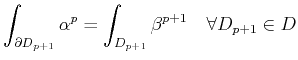
Another correspondence between cochains and ![]() -forms is given by the
concept of the coboundary operator. As introduced in Section
1.4.2, the coboundary operator is defined to
allow the transition from a topological equation of the form
-forms is given by the
concept of the coboundary operator. As introduced in Section
1.4.2, the coboundary operator is defined to
allow the transition from a topological equation of the form
| (1.55) |
to the following relation between cochains:
| (1.56) |
 |
(1.58) |
| (1.59) |
Given the properties of the coboundary operator ![]() , the exterior
differential
, the exterior
differential ![]() can be seen as the continuous counterpart
[53] of
can be seen as the continuous counterpart
[53] of ![]() . The following table depicts the
correspondence between discrete and continuous concepts
[35].
. The following table depicts the
correspondence between discrete and continuous concepts
[35].
| discrete setting | continuous setting | ||
|
|
|
||
| boundary of a |
|
|
boundary of a |
|
|
weighted |
||
| pairing of |
|
|
weighted |
| coboundary operator | exterior differential operator | ||
Based on these concepts, the local vector field representation
![]() becomes an ordinary
2-form
becomes an ordinary
2-form ![]() and the scalar field
and the scalar field ![]() a twisted 3-form
a twisted 3-form
![]() :
:
| (1.60) | |
| (1.61) |
It has to be noted, that the given differential form expression is
more general than the vector calculus notation due to the fact that
the expression is valid for
![]() ,
,
![]() and the
discrete chain and cochain representations automatically express the
type of the dimension with the general notion of:
and the
discrete chain and cochain representations automatically express the
type of the dimension with the general notion of:
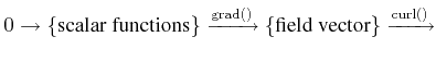
Examples of ![]() -form complexes for differential operators encountered
in different works [62,24]
for vector analysis in three dimensions are denoted by:
-form complexes for differential operators encountered
in different works [62,24]
for vector analysis in three dimensions are denoted by:
 |
(1.64) |
 |
The concept of constitutive links closes the gap between ordinary and twisted cochains with discrete links between them. Two different types can be obtained:
| (1.65) | ||
| (1.66) |
The inherently discrete computer implementation can now be equipped with all the necessary information and structure regarding the physical entities.