5.1 Generic Data Structures

The concepts given in Section 1.3, especially the cell topology and complex topology, are used here to derive a common specification of an interface to data structures. This specification is based on topological properties only and thereby separates the actual data storage structure from the stored data. In terms of the fiber bundle theory, generic data structures can be seen as modeling the base space. By the identification of the chain and cochain concepts (Section 1.4) within the fiber bundle concept (Section 1.6), the concepts presented here can also be seen as models for the chain concept with the intrinsic fibers of incidence information. The here given approach collects the incidence numbers [31,35] as well as the connection matrix [53].

The first step towards a generic data structure is the integration of the various already existing data structures. For example, Figure 5.1 presents the structure of a singly linked list.

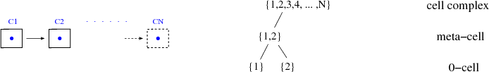
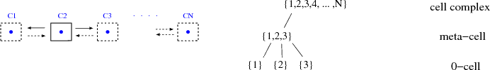
**Figure 5.1:** Complex topology of a singly linked list.
$\begin{figure}\begin{center} \epsfig{figure=figures/complextopology_sll.eps, width=16cm} \end{center} \end{figure}$

In terms of topological concepts, only locally neighboring cells can be traversed by this data structure, which can be seen by the representation of the complex topology by the poset on the right side. The number of elements in the meta-cell subsets is bounded by a constant number, unique for each type of data structure in the 0-cell complex regime, whereas the concept of a meta-cell is introduced in Section 1.3.3. The singly linked list uses two elements in the meta-cell, later declared as local(2) and called forward concept in the STL. The mechanisms used to describe the doubly linked list are the same as those used for the singly linked list. Compared to the singly linked list, three elements in the meta-cell are used, local(3), as can be seen in Figure 5.2. The concept of bidirectional traversal is used in the STL for this type of data structure. A binary tree data structure can also be modeled by this type of complex topology.

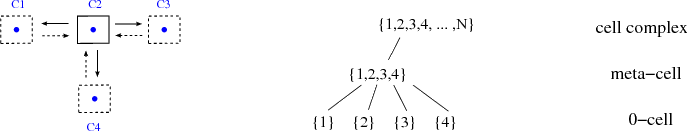
**Figure 5.2:** Complex topology of a doubly linked list.
$\begin{figure}\begin{center} \epsfig{figure=figures/complextopology_dll.eps, width=16cm} \end{center} \end{figure}$

Next, the complex topology of a tree structure is depicted in Figure 5.3, whereas the term local(4) is used for the characterization of the meta-cell. As can be seen, the singly linked list, the doubly linked list, and the tree contain a similar structure and differ only in the number of elements in their respective meta-cells.

**Figure 5.3:** Complex topology of a tree.
$\begin{figure}\begin{center} \epsfig{figure=figures/complextopology_tree.eps, width=16cm} \end{center} \end{figure}$

The last data structure related to commonly used structures within the 0-cell complex is based on the concept of an array. Its complex topology is shown in Figure 5.4. A notable difference with respect to the data structures which have already been reviewed can be observed. The poset is built by only two layers: the 0-cell sets and the complex set. This type of data structure therefore uses a so-called global property. All cells are directly accessible from the complex. In terms of the STL, this is called random access property.

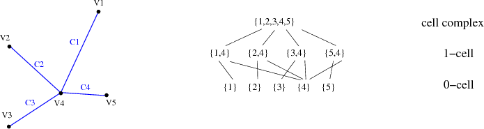
**Figure 5.4:** Complex topology of an array.
$\begin{figure}\begin{center} \epsfig{figure=figures/complextopology_array.eps, width=16cm} \end{center} \end{figure}$

The next example uses a cell dimension of one and therefore a one-dimensional cell complex. Figure 5.5 introduces the complex topology of this type of cell complex, commonly known as graph. Vertices incident to an edge as well as adjacent edges can be traversed.

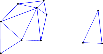
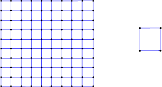
**Figure 5.5:** Complex topology of a graph.
$\begin{figure}\begin{center} \epsfig{figure=figures/complextopology_graph.eps, width=16cm} \end{center} \end{figure}$

These two types of complexes, the zero- and one-dimensional complexes, can now be abstracted into higher dimensional complexes with two different types of complex topologies: the local (Figure 5.6) and the global cell complex (Figure 5.7). Based on the cell complex types, the following cell types are available:

**Figure 5.6:** Local cell complex (left), normally called mesh, and a 2-cell representation (right). Vertices are marked with filled circles.
$\begin{figure}\begin{center} \epsfig{figure=figures/gsse_ncellcomplex1.eps, width=8cm} \end{center} \end{figure}$

**Figure 5.7:** Global cell complex (left), normally called grid, and a 2-cell representation (right).
$\begin{figure}\begin{center} \epsfig{figure=figures/gsse_ncellcomplex2.eps, width=7cm} \end{center}\vspace*{-0.2cm}\end{figure}$

The most important property of a CW-complex can be explained by the use of different

-cells and by consistently attaching sub-dimensional cells to the n-cells. In the following an abbreviation to specify the CW-complex with its dimensionality, e.g., a 1-cell complex describes a one-dimensional CW-complex, is used. So far all mechanisms to handle the underlying topological space of data structures have been introduced. Each subspace, the

-skeleton, can be uniquely characterized by its dimension. All these subspaces are connected appropriately by the concept of a finite CW-cell complex. The first part of the data structure characterization is listed in Table 5.1.

Table 5.1: Classification scheme based on the dimension of cells.

data structure	cell dimension
array	0
singly linked list (SLL) / stream	0
doubly linked list (DLL) / binary tree	0
arbitrary tree	0
graph	1
grid,mesh	2,3,4,..

A common scheme of characterizing data structures by their dimensions is now available. A drawback of this characterization can easily be seen by the 0-cell complexes. The topological space and subspaces only guarantee the correct connection of its subsets, but traversal mechanisms cannot be derived based on these concepts. Therefore, concepts of order theory, as given in Section 1.3.1, are used to formalize the internal structure of cells and the structure of a cell complex. Incidence traversal can then be directly derived from this concept.

The characterization given in Table 5.1 is extended with the cell topology in Table 5.2. The zero-dimensional cell complex types do not differ at all using this classification. But for dimensions greater than one, a distinction of cell topologies becomes apparent.

Table 5.2: Classification scheme based on the dimension of cells and the cell topology.

data structure	cell dimension	cell topology
array	0	simplex
SLL/stream	0	simplex
DLL/binary tree	0	simplex
arbitrary tree	0	simplex
graph	1	simplex
grid	2,3,4..	cuboid
mesh	2,3,4..	simplex

Based on the formal concepts just defined, the classification scheme can be further refined using the number of elements in the meta-cells. An overview is provided in Table 5.3. The complex topology uses the number of elements of the corresponding meta-cells.

Table 5.3: Classification scheme based on the dimension of cells, the cell topology, and the complex topology.

data structure	cell dimension	cell topology	complex topology
array/vector	0	simplex	global
SLL/stream	0	simplex	local(2)
DLL/binary tree	0	simplex	local(3)
arbitrary tree	0	simplex	local(4)
graph	1	simplex	local
grid	2,3,4,..	cuboid	global
mesh	2,3,4,..	simplex	local

This final classification scheme introduces a unique classification scheme based on topological properties only, where well-known and used data structures, e.g., a singly linked list, are also integrated. Thus the internal structure of data and traversal is clearly distinct from all quantity storage mechanisms.