As given in Section 1.6, the chain
concept can be used in conjunction with the fiber bundle concept, by
the so-called intrinsic incidence information of each ![]() -skeleton.
In this work, the information regarding the cell topology is stored
within the poset, where the complex topology information, for the
local case, has to be stored explicitly. To enable an efficient means
for this type of storage, an additional concept of a connection matrix
[53] is introduced not only to derive neighborhood
information of cells, but also to enable different types of traversal
mechanisms. To enable vertex-on-cell traversal, only the minimal
information has to be stored. To enable a full traversal hierarchy,
not only the vertex-on-cell but also the cell-on-vertex information
has to be stored. Based on this twofold incidence information, the
full hierarchy of traversal is available. It is also of utmost
importance to store the local orientation of each cell to avoid
additional implementation overhead for the subsequent applications.
-skeleton.
In this work, the information regarding the cell topology is stored
within the poset, where the complex topology information, for the
local case, has to be stored explicitly. To enable an efficient means
for this type of storage, an additional concept of a connection matrix
[53] is introduced not only to derive neighborhood
information of cells, but also to enable different types of traversal
mechanisms. To enable vertex-on-cell traversal, only the minimal
information has to be stored. To enable a full traversal hierarchy,
not only the vertex-on-cell but also the cell-on-vertex information
has to be stored. Based on this twofold incidence information, the
full hierarchy of traversal is available. It is also of utmost
importance to store the local orientation of each cell to avoid
additional implementation overhead for the subsequent applications.
The basic property for a consistent data structure is the total
ordering of the ![]()
![]() -cells of an
-cells of an ![]() -dimensional complex
-dimensional complex
![]() , whereas the vertices of a cell are modeled by a
partial ordering, as introduced in Section
1.3.1. Based on the lattice
property of a cell complex, which every complex in this work fulfills,
each cell can be uniquely identified by its set of vertices, e.g., a
, whereas the vertices of a cell are modeled by a
partial ordering, as introduced in Section
1.3.1. Based on the lattice
property of a cell complex, which every complex in this work fulfills,
each cell can be uniquely identified by its set of vertices, e.g., a
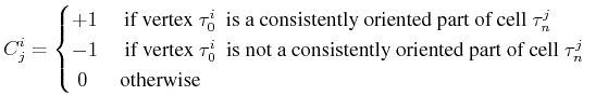
![]() -cell:
-cell:
| (5.2) |
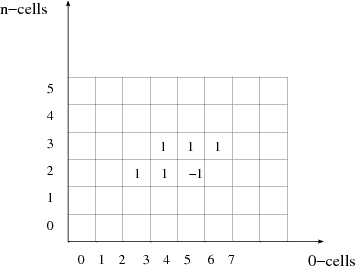
An example for a connection matrix is depicted in Figure 5.9, where the zeros are omitted, thus revealing the sparse structure of the matrix.
The connection matrix, obtained by a mesh generator, thereby enables the following traversal operations:
By using the poset mechanism and the stored orientation information to initialize the poset structure accordingly, the following additional traversal mechanism are available:
Using additional evaluation mechanisms of the connection matrix, adjacence traversal is also possible:
By evaluating the adjacence information, boundary operators can also be derived.