Subsections

• 7.2.1 Traversal Operators
• 7.2.2 Data Accessors
• 7.2.3 Arithmetic Functors
• 7.2.4 Domain-Specific Embedded Language

7.2 The Generic Functor Library

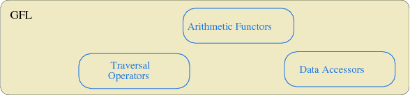
The GFL is the second important contribution of this work utilizing the concept of a DSEL (Section 4.3) to support functional programming in C++. The GFL is connected to the GTL only by means of topological traversal interfaces and quantity accessors, thereby providing mechanisms to separate discrete mathematics into topological and numerical operations by arithmetic functors. Figure 7.10 presents these building blocks of the GFL.

Figure 7.10: The generic functor library of the GSSE.

Based on this collection of functors and using the compile-time functional library Phoenix 2 [44], a highly efficient, maintainable, and scalable DSEL has been created. It is important to note that all functors can be used completely orthogonally with all other functors.

7.2.1 Traversal Operators

As can be seen in Section 7.1, the traversal operations require some additional code to create and initialize the iterators. To ease the application of the GTL, a traversal functor is realized, as given in the next code snippet

where cell_type_1 represents the base cell under consideration, whereas cell_type_2 specifies an incident sub-cell, e.g., a vertex or an adjacent cell. This mechanism can use virtually any derived internal structure of a cell or of the whole cell complex to build the requested traversal and avoids the construction and initialization specification. The following source snippet uses a given cell type and derives the boundary of this cell for traversal:

An example of this cell type is a 3-cuboid cell and generates the $3-1$ -cell traversal operation. In other words, this traversal operation generates a facet-on-cell iterator. Simple cell traversal can be specified by the following example which also demonstrates an even shorter specification for this special case:

Figure 7.11 provides examples of a simplex cell and complex type and reviews the possible relationships between topological elements of different dimensions. The first row shows all edges, faces, and cells which are incident with the same base vertex (a)-(c), while the first column shows vertices which are incident with one base edge, face, or cell (d, g, j).

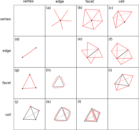Figure 7.11: Traversal methods induced by the incidence relation. The rows illustrate traversal schemes of the same base element, whereas columns depict traversal schemes of the same traversal element.

The connection matrix is the underlying data structure for these types of operations.

7.2.2 Data Accessors

An important concept is the evaluation of quantities related to given topological elements. For example, the quantity storage of discretization schemes requires the evaluation and access of several different dimensional quantity types, e.g., the finite volume method uses edge distances and areas as well as vertex quantities. To create an automatic evaluation of these different types of quantity access, the GFL implements generic data accessors which represent a C++ function object. This means that this object implements, on the one hand, a mechanism for automatic type deduction, and, on the other hand, the operator(). In the following code snippet a simple example of the generic use of this accessor is given, where a scalar value is assigned to each vertex in a domain. The quantity accessor creates an assignment which is passed to the std::for_each algorithm.

7.2.3 Arithmetic Functors

The discretization schemes, as well as several other methods, require standard arithmetic operations. Therefore generic calculations are necessary which can be specified with the corresponding arithmetic operation. The GFL implements comprehensive functor mechanisms. Using these mechanisms as a foundation, the following two algebraic generic components were developed, which are sufficient for all discrete representations of the operations of integration and differentiation. Additionally it is necessary that this generic calculation automatically deduces the neutral element of the given operator for initialization.

Shortcuts are also available for these common operations:

7.2.4 Domain-Specific Embedded Language

A domain-specific embedded language based on the given building blocks of generic traversal, data accessors, and arithmetic functors, as introduced in Section 4.3, is available.

To illustrate the application of the GFL in detail, a simple equation $\sum_{v\rightarrow e} (\Delta_{e\rightarrow v} \mathrm{u}) = 0$ is used where $\mathrm{u}$ denotes the quantity located on a vertex and $\Delta$ denotes the difference, whereas ${v\rightarrow e}$ states the traversal operation. To express the difference between imperative and functional programming, the example is presented first without the GFL. For both programming paradigms it can be seen that this implementation does not depend on the dimension or type of the cell complex.

The same functionality is obtained by using the functional programming paradigm. The main difference is given by the absence of temporary variables within the functional style.

The complex resulting from this mapping is completed by specifying the current vertex object *vit at run-time, which clearly demonstrates the compile-time and run-time border. For a comprehensive explanation the specific parts are separated. The first part specifies a traversal of all vertices in an imperative way.

The following bracket encompass the actual functional expression. The *vit represents the currently evaluated terminal object, in this case a dereferenced vertex.

The heart of the equation is shown in the next code snippet. Here a sum is used as the discrete representation of the arithmetic operator. The topological traversal is given by the vertices incident to the edge. This inner part receives the edge information from the sum<vertex,edge> and builds a traversal on the vertices on this edge.

The quantity accessor u supplies the sum algorithm with values stored on the vertices. Finally, the summed value obtained from all operations within sum is stored in the object eq. To show maintainability and scalability, an example of a discretized form of the Laplace equation is given:

$$\mathcal{L}_\mathrm{ell\_fv}({\ensuremath{\mathrm{u}}}) \equiv \s... ...lta_{e\rightarrow v} {\ensuremath{\mathrm{u}}}) \frac{A}{d} \varepsilon= 0 \; ,$$

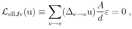where ${\ensuremath{\mathrm{u}}}$ denotes the solution quantity and $\Delta$ again denotes the difference. The geometrical factors $A$ and $d$ , necessary for the finite volume discretization approach, denote the cross section of the flux and the distance between the two edge points, respectively. The final source code reads:

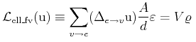
With small changes the Laplace equation can be extended to a Poisson equation:

$$\mathcal{L}_\mathrm{ell\_fv}({\ensuremath{\mathrm{u}}}) \equiv \s... ...rightarrow v} {\ensuremath{\mathrm{u}}}) \frac{A}{d} \varepsilon = V \varrho \;$$

In the next code snippet, the functional character of the implementation approach and the resulting extensibility, is given. Most of the source code remains unchanged; only minor parts have to be added.

The non-zero right-hand side of the Poisson equation leads to a multiplication with the volume $V$ when the integration is performed using finite volumes.