Maxwell's equations, given in Section 1.2,
are the basic equations for the examples given here. For the
stationary electrostatical case, the time derivatives vanish and
![]() is obtained. Such an equation can be expressed by a
scalar potential
is obtained. Such an equation can be expressed by a
scalar potential
![]() which is
subsequently used to derive the capacitance and resistance analysis
[114].
which is
subsequently used to derive the capacitance and resistance analysis
[114].
For the given stationary case with linear dielectric, the ratio of
charge ![]() and voltage
and voltage ![]() of conductors is constant and is called
capacitance
of conductors is constant and is called
capacitance
![]() . Due to the fact that the inner part of
the conductors is free of electric field, the charge is distributed
only on their surfaces. The charge distribution is derived from
. Due to the fact that the inner part of
the conductors is free of electric field, the charge is distributed
only on their surfaces. The charge distribution is derived from
![]() by means of a surface charge
by means of a surface charge ![]() as given in Section
1.2 and Equation 1.13.
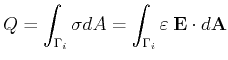
By integration of the charge on the surface of the conductor
as given in Section
1.2 and Equation 1.13.
By integration of the charge on the surface of the conductor
![]() the following is obtained:
the following is obtained:
 |
(9.1) |
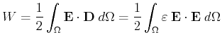
Then the capacitance ![]() can be derived. Another way can be described
by the energy method, where the stored energy is given by
can be derived. Another way can be described
by the energy method, where the stored energy is given by
![]() expressed in local field terms:
expressed in local field terms:
 |
(9.2) |
Here, the calculation domain covers the complete dielectric part and expands, theoretically, into infinite space. Therefore it is important to emphasize that most of the field energy is contained near the conductors, and so only a small part of the integration domain has to be covered [114].
Both of these calculation mechanisms require the calculation of the
electric field
![]() , where the charge integration requires only
the field at the surface of the conductor, which can be expressed by a
scalar potential
, where the charge integration requires only
the field at the surface of the conductor, which can be expressed by a
scalar potential
![]() . The Maxwell equation
. The Maxwell equation
![]() , and the fact that an isolator does not
carry electric charge (
, and the fact that an isolator does not
carry electric charge (
![]() ), the following equations are
used to determine a potential distribution as well as for the
extraction of the capacity of a given domain:
), the following equations are
used to determine a potential distribution as well as for the
extraction of the capacity of a given domain:
| (9.3) | ||
| (9.4) | ||
| (9.5) |
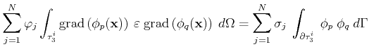
As introduced in Section 2.3, the
finite element formulation is represented by the following equation system for ![]() -elements:
-elements:
where the following expression for the charge distribution is
used
![]() . This problem is
linear and the global system matrix is simply obtained by assembling
. This problem is
linear and the global system matrix is simply obtained by assembling
![]() with the corresponding node index transformation into the global
matrix.
with the corresponding node index transformation into the global
matrix.
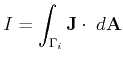
The electric resistance can be described by the global law
![]() . The resistance of a conductor can then be calculated
by using a potential on the boundary of this conductor and calculating
the current by an integration of an area of conductor
. The resistance of a conductor can then be calculated
by using a potential on the boundary of this conductor and calculating
the current by an integration of an area of conductor
![]() :
:
 |
(9.7) |
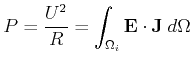
or by calculating the electrical power loss:
 |
(9.8) |
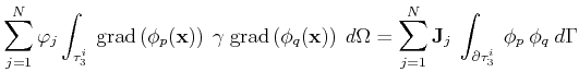
Similar to the capacitance calculation, the electric field
![]() has to be calculated. The lack of sources of the electrical current
density
has to be calculated. The lack of sources of the electrical current
density
![]() in the electrostatic system is also
retained. Then the following equation for the current density is
obtained, where
in the electrostatic system is also
retained. Then the following equation for the current density is
obtained, where
![]() is the inside of a current-carrying
conductor:
is the inside of a current-carrying
conductor:
| (9.9) | ||
| (9.10) | ||
| (9.11) |
To obtain the global solution, a procedure where all the local
matrices have to be inserted into the global system matrix
![]() is used, called assembly. Equation
9.6 as well as Equation
9.12 evaluated on all elements of
a domain can then be expressed by a matrix notation:
is used, called assembly. Equation
9.6 as well as Equation
9.12 evaluated on all elements of
a domain can then be expressed by a matrix notation:
where
![]() is the global system matrix,
is the global system matrix,
![]() the
solution vector, and
the
solution vector, and
![]() the right-hand side. A transformation
of the local indices to global indices is required to obtain
consistent system matrix entries.
the right-hand side. A transformation
of the local indices to global indices is required to obtain
consistent system matrix entries.
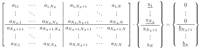
The right-hand side matrix
![]() is obtained by contributions of
elements on the boundary of the domain, thereby only containing values
not equal to zero for boundary contact nodes. A detailed notation of
Equation 9.13 is given by [114]:
is obtained by contributions of
elements on the boundary of the domain, thereby only containing values
not equal to zero for boundary contact nodes. A detailed notation of
Equation 9.13 is given by [114]:
 |
(9.14) |
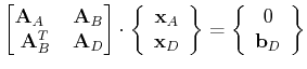
where the upper half corresponds to the inner nodes whereas the lower half can be identified by the boundary nodes. The unknown values are underlined. Expressed as block matrices the equation system reads:
 |
(9.15) |
To obtain the unknown values
![]() inside the domain, the
equation system has to be solved:
inside the domain, the
equation system has to be solved:
| (9.16) |
The electric charge is then obtained by:
| (9.17) |
| (9.18) |
The transformation of the given expression is supported by GSSE's finite element components, given in Section 7.3.4. The following set of operations is required to obtain the solution:
Where the first step is already implemented in the GSSE . The second and third step are given in the following source snippet for two- and three-dimensional simplex and cuboid cell complexes:
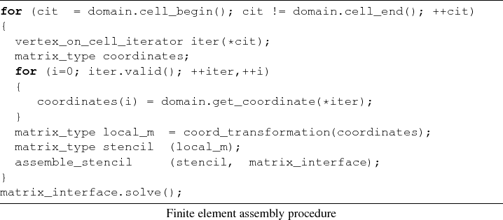
The final line invokes the solver using the generic solver interface.
Because of the library-centric application design approach of the GSSE
and the derived applications, the matrix_type can be
implemented by any matrix data structures, e.g., the high performance
Blitz++ [150] matrices, or the C++
valarray. A performance comparison is given in Section
7.4.