4.5.3 Point Response Interface

As already mentioned in Sec. 3.2 it is possible to efficiently combine the abilities of an analytical ion implantation simulator with a Monte-Carlo ion implantation simulator. Therefore a representative point response function can be calculated by the Monte-Carlo simulator .

A small window has to be defined as an implantation window around a representative point. A point response function is defined as the implanted distribution resulting from an implantation through a single point of the surface. But for the calculation of a point response function the size of the implantation window must not be too small. Even if this is contrary to the definition it has to be mentioned that in case of a too small window the de-channeling effect is underestimated, because the damage concentration decreases in the horizontal direction when a point response function is calculated, while it is constant if the complete simulation domain is implanted. A lowered damage concentration results in a reduced de-channeling probability (Sec. 3.3.5) which influences also the doping distribution. The larger the implantation window the less this boundary effects contribute to the total particle distribution. Thereby the accuracy of the calculated response function increases.

By default the representative point is assumed to be in the middle of the surface of the simulation domain and the size of the implantation window is three times the estimated projected range of the implanted particles. This window size has turned out to be good compromise between minimizing the implantation window (reduced computation time) and accurately treating the damage accumulation .

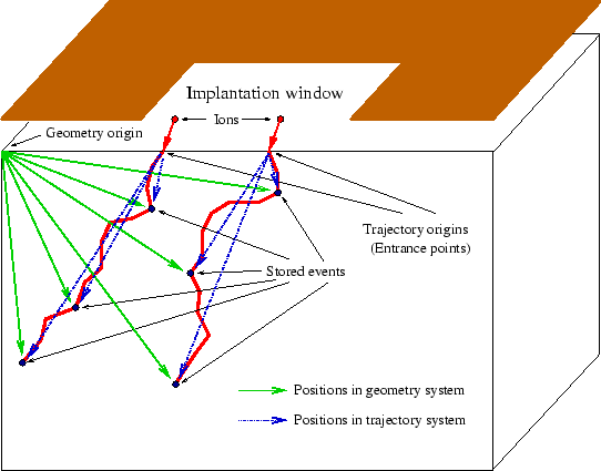
As already mentioned the drawback of using a large implantation window is, that not a real point response function is calculated but a smeared point response profile according to the finite size of the implantation window. The point response compression method presented in the following is capable to overcome this problem without loosing damage information. A schematic description how the compression method derives a real point response function from the originally calculated distribution is presented in Fig. 4.10.

Figure 4.10: Illustration how the point response compression method works.

In principle the point response compression method transforms the simulation results from a coordinate system connected to the simulation domain to a coordinate system related to the entrance point of an ion trajectory.

Figure 4.11: Two cuts through a compressed (top) and an uncompressed (bottom) point response function resulting from an implantation into crystalline silicon covered with 15 nm silicon dioxide. An implantation window with a size of 300 nm was used.

Whenever simulation data like damage information or doping information are generated they have to be stored in a histogram representing all simulation results. The input provided for storing information is the location of the new data and the value that has to be added to a histogram element which contains the specified location. In order to create a compressed point response function each event is stored twice. On the one hand it is stored in a simulation histogram using the original position for storing and on the other hand it is stored in a point response histogram with a position relative to the entrance point of the ion into the simulation domain. The point response histogram is only used for storing data, while all information which influences the trajectory calculation, like the previously accumulated damage, is taken from the simulation histogram.

By using the relative position to the entrance point for storing data in the response histogram the stored simulation results seem to be generated by ions entering the simulation domain through a single point. Since the entrance point in the real coordinate system is related to the origin in the coordinate system of the response histogram all ions seem to enter through the origin of the coordinate system. Therefore the resulting distribution function equals the definition of a point response function. Just the implantation dose is not represented correctly, but anyway, the specification of a dose makes no sense for a point response function because it has to fulfill the normalization condition (3.1). Fig. 4.11 shows two cuts through a compressed and an uncompressed point response function resulting for an implantation into crystalline silicon covered with 15 nm silicon dioxide with boron ions with an energy of 70 keV and a dose of $4{\cdot }10^{15}$cm$^{-2}$. An implantation window with a size of 300 nm was used for the calculation and the ion beam was tilted by 7 $\,^\circ\;$.

In order to demonstrate the influence of the size of the implantation window on the calculated point response function three iso-lines of four point response functions are compared in a cut-plane containing the origin and being perpendicular to the x-axis in Fig. 4.14. The point response functions are generated by using implantation windows with sizes of 50 nm, 100 nm, 200 nm and 300 nm.

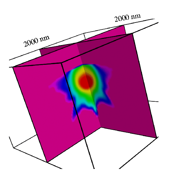
The three-dimensional structure of a compressed Monte-Carlo point response function is shown in Fig. 4.12 and Fig. 4.13 where iso-surfaces of point response functions resulting from implantations with boron ions with energies of 40 keV an 70 keV and with doses of $5{\cdot }10^{14}$cm$^{-2}$ and $4{\cdot }10^{15}$cm$^{-2}$ are presented. In both cases the ion beam is tilted by 7 $\,^\circ\;$and the input structure is a crystalline silicon substrate covered with 15 nm silicon dioxide.

Figure 4.12: Two iso-surfaces ( $1{\cdot }10^{17}$cm$^{-3}$ (a) and $1{\cdot }10^{18}$cm$^{-3}$ (b)) of a compressed point response function resulting from an implantation into crystalline silicon covered with 15 nm silicon dioxide with boron ions with an energy of 70 keV and a dose of $4{\cdot }10^{15}$cm$^{-2}$.

Figure 4.13: Two iso-surfaces ( $1{\cdot }10^{17}$cm$^{-3}$ (a) and $1{\cdot }10^{18}$cm$^{-3}$ (b)) of a compressed point response function resulting from an implantation into crystalline silicon covered with 15 nm silicon dioxide with boron ions with an energy of 40 keV and a dose of $5{\cdot }10^{14}$cm$^{-2}$.

Figure 4.14: Comparison of three iso-lines ( $5{\cdot }10^{19}$cm$^{-3}$, $5{\cdot }10^{18}$cm$^{-3}$ and $5{\cdot }10^{17}$cm$^{-3}$) for point response functions generated by using implantation windows with sizes of 50 nm, 100 nm, 200 nm and 300 nm.

Figure 4.15: Header of a point response file.

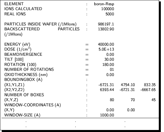
After finishing a point response simulation besides the normal output several additional files containing the calculated point response functions are produced. At least three point response functions are generated by one Monte-Carlo simulation run, one for each implanted particle species, one for the interstitial distribution and one for the vacancy distribution . Besides the point response distribution function which is represented on an ortho-grid lined up with the coordinate system of the simulation domain, a header is added to the point response file containing some additional information for the analytical implantation simulator IMP3D like the implantation conditions, a description of the implantation window and of the data histogram .

Footnotes

... simulator

The command-line parameter pointResponse determines that a point response function is calculated.

... accumulation

The user can override the default setting for the implantation window by explicitly specifying an implantation window by the command-line parameter implantationWindow.

... distribution

The filenames are derived from the name of the simulation output file, by adding the species name and the extension -Resp-RESP.DAT. For instance if the output name is Output.pbf a point response file with the name Output_boron-Resp-RESP.DAT is generated.

... histogram

The value of the parameter oxidthickness in the point response file header is determined by the command-line parameter oxideThickness. This parameter has no influence on the behavior of MCIMPL, it is just used by the analytical ion implantation simulator to characterize the implantation conditions.