7.2 Stress Calculation Concept for Simulation

Normally only a small part of the whole real structure is investigated by simulation because of limited computer resources and desired short simulation times. Mostly the simulation of this small part delivers the needed information, because most structures have only few areas of interest or they are repeating. Therefore, also for the oxidation process the simulated domain is a three-dimensional cut of the complete structure.

Figure 7.1: Structure with plain side walls for oxidation simulation.

Figure 7.2: Side walls are restricted in movements to avoid their deformations.

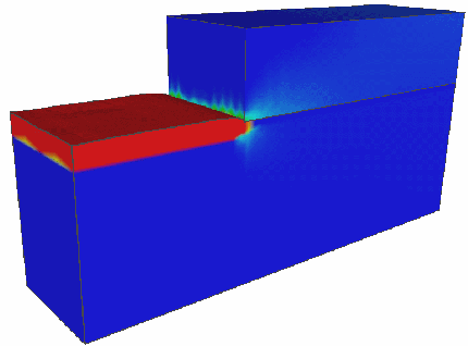
Such a cut is shown in Fig. 7.1. This example represents a piece of the silicon substrate with (1.2$\times$0.3) $\mu$m floor space where two thirds of the length are covered with a 0.15 $\mu$m thick silicon nitride mask. Only the upper surface has contact with the oxidizing ambient. The body has plain side walls which must not be deformed by simulation. This means that the four side walls are not allowed to move in their normal directions, as demonstrated in Fig. 7.2.

For the 125% additional volume of the newly formed oxide in (7.8) an isotropic expansion is assumed. This means that all strain components $\varepsilon_{0,ii}$ are equal. Because of the prevented movements of the simulation domain in the normal directions of the side walls the volume can not expand in the xy-plane, only in z-direction. The mechanical boundary conditions and the isotropic approach build up an enormous stress (pressure) in the whole oxide layer (see Fig. 7.3). In the mathematical formulation (7.7) this effect can be explained by the fact that $\varepsilon_{xx}=\varepsilon_{yy}=0$.

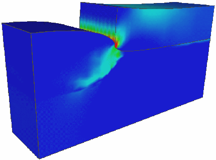
The resulting high pressure all over the new generated oxide layer has the fatal effect on stress dependent simulation that the oxidation process is de facto stalled after a few time steps. The high pressure in the SiO$_2$-layer is in principle a wall for oxidant diffusion and chemical reaction, because both are decreased exponentially with pressure. Thereby, even for a long oxidation time the oxide thickness is minimal (see Fig. 7.3), and so the simulation results are totally wrong.

Figure 7.3: High pressure in the whole oxide layer due to isotropic expanding approach.

A possibility to solve this problem starts with the following considerations. For a plain surface (xy-plane) which is oxidized the oxide nearly grows stress-free only in the normal z-direction. In that case the isotropic approach for the volume increase is not correct, because it should be $\varepsilon_{0,xx}=\varepsilon_{0,yy}=0$ and $\varepsilon_{0,zz}=V^{add}_{rel}$ in order to get the correct displacements of the new oxide in z-direction. For this purpose the isotropic approach should be modified. The question is how this can be performed automatically, because the displacements $\vec{d}$ are the results of the mechanical problem and the strains $\varepsilon_{0,ii}$ are the inputs. On the other side for the simulation of different structures the isotropic approach is the most general one.

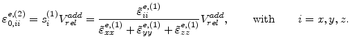
It was found that the best strategy is to calculate the displacements in two steps. In the first step, denoted with ${}^{(1)}$, the displacements $\vec{d}^{e,(1)}$ on a finite element are calculated with the universal isotropic approach

$$\varepsilon_{0,xx}^{e,(1)}=\varepsilon_{0,yy}^{e,(1)}=\varepsilon_{0,zz}^{e,(1)}=\frac{{}_1}{{}^3}V^{add}_{rel},$$ (7.14)

The actual strains for the first step can be calculated after solving the mechanical problem with the results $\vec{d}^{e,(1)}$ by

$$\tilde{\varepsilon}^{e,(1)} = \mathbf{B} \vec{d}^{e,(1)}.$$ (7.15)

The idea now is to use these strains from the first step to load the mechanical problem for the second step. The actual strain components $\tilde{\varepsilon}_{ii}^{e,(1)}$ show in which directions the volume of a finite element can expand easily and in which ones it can extend hardly or is even blocked ( $\tilde{\varepsilon}_{ii}^{e,(1)}=0$). The actual expansion $s_i$ in each direction $x$, $y$, and $z$ can then be expressed by

$$s_i^{(1)}=\frac{\tilde{\varepsilon}^{e,(1)}_{ii}}{\tilde{\varepsi... ...e,(1)}_{yy}+\tilde{\varepsilon}^{e,(1)}_{zz}}\qquad\mathrm{with}\qquad i=x,y,z.$$ (7.16)

As example it is assumed that $s_x=0$, $s_y=0.2$, and $s_z=0.8$. This means that the volume expansion is blocked in $x$- and prevented in $y$-direction. In $z$-direction there is the least resistance and so 80% of the actual volume increase happens there.

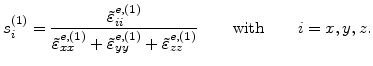
The minimal pressure in the elements can be reached, if the ratio of the input strains $\varepsilon_{0,ii}$ is the same as the percentage of the actual expansions $s_i$, because the ratio of the input strain components would be the same like the percentage of possible volume expansion in each direction. Therefore, the input strains for the second mechanical step are exactly weighted with the actual expansions from the first step in oder to get a minimal pressure in the increasing volume

$$\varepsilon_{0,ii}^{e,(2)}= s_i^{(1)}V^{add}_{rel} =\frac{\tilde{... ...ilde{\varepsilon}^{e,(1)}_{zz}}V^{add}_{rel},\qquad\mathrm{with}\qquad i=x,y,z.$$ (7.17)

The strains $\tilde{\varepsilon_0}^{e,(2)}$ load the mechanical problem with (7.9) for the second step. After solving the mechanical system again with (7.16) the actual strains $\tilde{\varepsilon}^{e,(2)}$ and therefore the final stress (pressure) for each finite element can be found with the conventional stress formula

$$\tilde{\sigma}^e = \mathbf{D} (\tilde{\varepsilon}^{e,(2)} - \tilde{\varepsilon_0}^{e,(2)}) + \tilde{\sigma_0}^e.$$ (7.18)

With the above described two-step stress calculation concept the pressure distribution in the simulated oxide domain meets the real physical conditions, as demonstrated in Fig. 7.4, because it avoids unnatural stresses which only come from the inappropriate modeling approach (isotropic expansion approach) and a simulation effect (cut structure where the side walls are not allowed to move in normal direction).

Figure 7.4: Pressure distribution with the two-step stress calculation concept.

Therefore, with this method and its right pressure distribution, the simulation with stress dependent parameters is treated properly, as displayed in Fig. 6.10.