Subsections

• 8.1.1 Electro-Thermal Simulation
• 8.1.2 Thermo-Mechanical Stress Simulation

8.1 Simulation Procedure

Thermo-mechanical simulation demands a temperature distribution in the structure. It was found out that the electrical characteristics of the complete system do not considerably change with stress during standard operation. Therefore, the simulation can be separated into an electro-thermal and a thermo-mechanical part within small time periods as long as there is no void nucleation in the interconnect lines or the passivation is not broken.

In the simulation sequence as displayed in Fig. 8.1, the first part is the three-dimensional transient electro-thermal simulation of the interconnect structure in order to calculate the temperature distribution. Additionally this simulation delivers the potential and the current density. With the temperature distribution from the first part, the three-dimensional thermo-mechanical simulation can be performed subsequently. With the electro-thermal and the thermo-mechanical simulation all necessary capabilities for the rigorous simulation of electromigration are available.

Figure 8.1: Simulation sequence and data flow.

For the electro-thermal investigation the simulator STAP [124] from the Smart Analysis Programs package, which has also been developed at the Institute for Microelectronics, is used. The other simulations can be carried out by the diffusion and oxidation simulator FEDOS. For the straightforward data exchange between the different simulators, WSS files are used, because STAP as well as FEDOS can handle the WSS format.

Although STAP is also based on FEM, it is not appropriate to use it for thermo-mechanical simulations, because STAP is specialized and optimized for fast and accurate electro-thermal simulations. An extension of STAP to a more universal tool which can also handle mechanical problems would reduce its performance significantly. So even with the necessary data exchange the decoupled simulations with STAP and FEDOS are more efficient than a coupled simulation only performed by STAP.

8.1.1 Electro-Thermal Simulation

The electro-thermal simulation is performed with the simulator STAP which uses also the finite element method for the calculation of the electric potential and temperature distribution. For the numerical calculation of Joule self-heating effects, caused by the electric current flow through the wire, two partial differential equations have to be solved [125,126]. The first one describes the electric subproblem

$$\mathrm{div}(\gamma_E\; \mathrm{grad} {\varphi}) = 0.$$ (8.1)

The electric potential $\varphi$ needs to be solved only inside domains composed of electrically conducting material ($\gamma_E$ represents the electrical conductivity). On the surface of the conductors three types of boundary conditions are allowed:

$\bullet\;$ Dirichlet - a constant potential is specified
$\bullet\;$ Neumann - vanishing current density is specified
$\bullet\;$ Floating potential - the total current is specified and the potential is forced to be the same all over the boundary area.

The next step is to compute the power loss density $p_D$ described by

$$p_D=\gamma_E\; (\mathrm{grad} \varphi)^2.$$ (8.2)

In addition the heat conduction equation has to be solved in order to obtain the distribution of the temperature $T$ in the whole interconnect structure

$$\mathrm{div}(\gamma_T\; \mathrm{grad} T)=c_p \rho_m\frac{\partial T}{\partial t}-p_D,$$ (8.3)

where $\gamma_T$ represents the thermal conductivity, $c_p$ the specific heat, and $\rho_m$ the mass density.

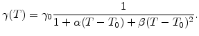
The temperature dependence of the thermal and electrical conductivities is modeled with second order approximations:

$$\gamma(T)=\gamma_0\frac{1}{1+\alpha(T-T_0)+\beta(T-T_0)^2}.$$ (8.4)

In (8.4) $\gamma_0$ is the electrical or thermal conductivity at a temperature $T_0$ of 300 K, $\alpha$ and $\beta$ are the linear and quadratic temperature coefficients. This makes the problem non-linear. Since the non-linearity is relatively weak, a simple iterative relaxation method is used which quickly converges to the solution, usually after 3-6 iterations.

8.1.2 Thermo-Mechanical Stress Simulation

High tensile stresses in the copper interconnects can cause break-up of the material and development of voids [127]. On the other side compressive stresses can induce the generation of extrusions. In case of temperature changes thermo-mechanical stress is build up because of (significant) different thermal expansion coefficients of adjacent materials.

The thermo-mechanical stress simulation is carried out with the program package FEDOS. The modeling of thermo-mechanical stress is similar to the stress calculation during thermal oxidation as described in Section 7.1. For the assumed elastic materials the stress tensor can be written in the form

$$\tilde{\sigma} = \mathbf{D} (\tilde{\varepsilon} - \tilde{\varepsilon_0}) + \tilde{\sigma_0}.$$ (8.5)

The main components of the residual stress tensor $\tilde{\varepsilon_0}$ include the desired volume change of the material caused by the temperature change. The strain components $\varepsilon_{0,ii}$ ($i$ stands for $x$, $y$, and $z$) are linearly proportional to the temperature $T$ in the material

$$\varepsilon_{0,ii}=\alpha_m (T-T_0),$$ (8.6)

where $\alpha_m$ is the thermal expansion coefficient for the respective material and $T_0$ is the ambient temperature assumed with 300 K.

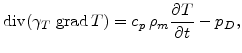
The temperature change loads the mechanical problem $\mathbf{K^e} \vec{d^e}=\vec{f^e}$ on every finite element, because the internal force vector is

$$\vec{f^e_{int}}=\mathbf{B^T}\mathbf{D} \tilde{\varepsilon_0}^e V^e.$$ (8.7)

The actual displacements $\vec{d}^e$ are obtained after solving the linear global equation system for the mechanics. With these results the actual strains can be calculated with $\tilde{\varepsilon}^e = \mathbf{B} \vec{d}^e$ and so the stress on an element can be determined with (8.5).

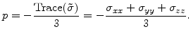
With the stress in principle also the hydrostatic pressure is given with the formula

$$p = - \frac{\mathrm{Trace(}\tilde{\sigma}\mathrm{)}}{3}= - \frac{\sigma_{xx}+\sigma_{yy}+\sigma_{zz}}{3}.$$ (8.8)