2.2.3 Electro-Magnetic Power Density

The local power density is one of the most important quantities that determine the maximum performance or the maximum number of device operations per time. Moreover, power has been concentrated at certain local regions and has therefore to be controlled appropriately to perform the desired action within the defined requirements. Unfortunately, power has also a dissipative part. Since the electrical and mechanical systems have only finite efficiencies, the usable power is less than the total power consumption. The difference dissipates via thermal conduction, convection, and radiation. In addition to that, the second law of thermodynamics postulates the irreversibility of some of the thermally dissipated heat. Hence, the entropy is steadily increasing on average. The appropriate power density for heat conduction can be derived from the local energy of the electro-magnetic fields, where the energy of these fields is determined by the POYNTING^2.21vector. The spatial power source density of the POYNTING vector represents the local energy density [58,59], which can be directly derived from the curl equations of MAXWELL's equations. Multiplying the equations (2.1) and (2.2) from the left with $-{\mathbf{{H}}}$ and ${\mathbf{{E}}}$ , respectively, results in

$$-{\mathbf{{H}}} \cdot (\nabla \times {\mathbf{{E}}}) {=}{\mathbf{{H}}} \cdot {{\partial}_{t}} {\mathbf{{B}}},$$ (2.84)

$${\mathbf{{E}}} \cdot (\nabla \times {\mathbf{{H}}}) {=}{\mathbf{{E}}} \cdot {\mathbf{{J}}} + {\mathbf{{E}}} \cdot {{\partial}_{t}}{\mathbf{{B}}}.$$ (2.85)

The sum of the left sides of equations (2.84) and (2.85) shows the local source density of POYNTING's vector:

$${\mathbf{{E}}} \cdot (\nabla \times {\mathbf{{H}}}) -{\mathbf{{H}... ...{{E}}} \times {\mathbf{{H}}}) {=}{{{{\boldmath {\nabla}}}}\cdot}{\mathbf{{S}}},$$ (2.86)

with the POYNTING vector ${\mathbf{{S}}}$ as

$${\mathbf{{S}}} {=}{\mathbf{{E}}} \times {\mathbf{{H}}}.$$ (2.87)

The sum of the right sides of equations (2.84) and (2.85) represents the equivalents to (2.86):

$${{{{\boldmath {\nabla}}}}\cdot}{\mathbf{{S}}} {=}{\mathbf{{E}}} \... ...tial}_{t}}{\mathbf{{D}}} + {\mathbf{{H}}} \cdot {{\partial}_{t}}{\mathbf{{B}}}.$$ (2.88)

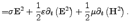
Equation (2.88) represents the local form of the energy conservation equation. The left side of (2.88) shows the local source density of the POYNTING vector which depicts the current change of energy density per time (power density). The right side shows the different components of the contribution. The first term ${\mathbf{{E}}} \cdot {\mathbf{{J}}}$ is the electric component which represents the JOULE power loss that causes self-heating due to carrier transport^2.22mechanisms. The second and the third term depict the change of the energy stored in the electrical and the magnetical field, respectively.

For isotropic and field-independent materials, (2.88) can be formulated as

$${{{{\boldmath {\nabla}}}}\cdot}{\mathbf{{S}}} {=}\sigma {\mathbf{... ...l}_{t}}{\mathbf{{E}}} + \mu {\mathbf{{H}}} \cdot {{\partial}_{t}}{\mathbf{{H}}}$$

$$%\label{eq:poynt6}\\ {=}\sigma {\mathbf{{E}}}^2 + {{\frac{1}{2}}... ... {{\frac{1}{2}}}\mu {{\partial}_{t}}\displaystyle\left({\mathbf{{H}}}^2\right).$$ (2.89)

With JOULE's power loss equation

$$p {=}{\mathbf{{E}}} \cdot {\mathbf{{J}}} {=}\sigma {\mathbf{{E}}}^2,$$ (2.90)

and the introduction of ${w^{\mathrm{el}}}$ and ${w^{\mathrm{mag}}}$ as the electrical and magnetical energy densities

$${w^{\mathrm{el}}}{=}{{\frac{1}{2}}}\varepsilon {\mathbf{{E}}}^2$$ (2.91)

$${w^{\mathrm{mag}}}{=}{{\frac{1}{2}}}\mu {\mathbf{{H}}}^2,$$ (2.92)

equation (2.89) can be written as

$${{{{\boldmath {\nabla}}}}\cdot}{\mathbf{{S}}} {=}p + {{\partial}_{t}}{w^{\mathrm{el}}}+ {{\partial}_{t}}{w^{\mathrm{mag}}}.$$ (2.93)

In comparison with common effects in semiconductor devices, JOULE's power loss has often to be taken into account to describe self-heating. In conjunction with semiconductor devices, there are several other approaches to determine the power loss. Since electrons and holes behave differently in semiconductor materials, the current is conveniently split up in order to account for their different properties. In addition, the potential confinement of the carriers is also different. Therefore, the power densities for electrons and holes can be determined with the appropriate models.