Next: 2.3 Electron Transport
Up: 2.2 Silicon
Previous: 2.2.1 Electronic Structure
Contents
For the calculation of the phononic bandstructure of silicon-based nanostructures, we employ the modified valence force filed method [45]. In this method the interatomic potential is modeled by the following bond deformations: bond stretching, bond bending, cross bond stretching, cross bond bending stretching, and coplanar bond bending interactions [45]. The model accurately captures the bulk silicon phonon spectrum as well as the effects of confinement [39]. In the MVFF method, the total potential energy of the system is defined as [39]:
![$\displaystyle U\approx \frac{1}{2}\sum_{i\in N_{\mathrm{A}}} \left[ \sum_{j\in ...
...right) +\sum_{j,k,l\in COP_i}^{j\neq k\neq l} U_{\mathrm{bb-bb}}^{jikl} \right]$](img198.png) |
(2.18) |
where
 ,
,  , and
, and  are the number of atoms in the system, the number of the nearest neighbors of a specific atom
  , and the coplanar atom groups for atom
, respectively. As shown in Fig. 2.5,
, and the coplanar atom groups for atom
, respectively. As shown in Fig. 2.5,
 ,
,
 ,
,
 ,
,
 , and
, and
 are the bond stretching, bond bending,
cross bond stretching, cross bond bending stretching, and coplanar bond bending interactions,
respectively [45,39]. The terms
,
, and
are an addition to the usual Keating
valence force filed (KVFF) model [48], which can only capture the silicon phononic bandstructure in a limited part of the Brillouin zone. As indicated in Ref. [39] the introduction of these additional terms provides a more accurate description of the entire Brillouin zone.
are the bond stretching, bond bending,
cross bond stretching, cross bond bending stretching, and coplanar bond bending interactions,
respectively [45,39]. The terms
,
, and
are an addition to the usual Keating
valence force filed (KVFF) model [48], which can only capture the silicon phononic bandstructure in a limited part of the Brillouin zone. As indicated in Ref. [39] the introduction of these additional terms provides a more accurate description of the entire Brillouin zone.
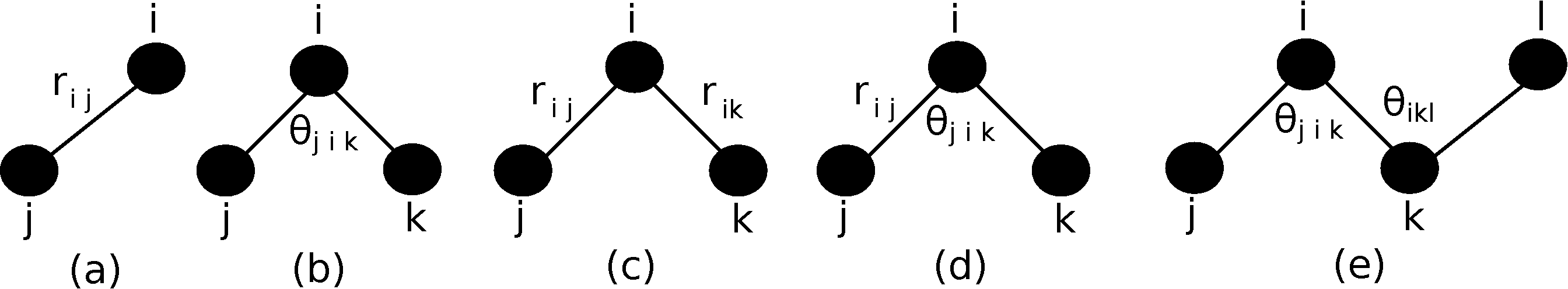
Figure 2.5:
Schematic representation of (a) bond-stretching, (b) bond bending, (c) cross bond stretching, (d) cross bond bending-stretching, and (e) coplanar bond bending interactions.
|
|
These short-range interactions depends on the atomic positions by [39]:
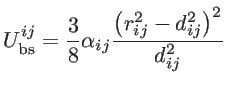 |
(2.19) |
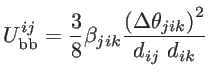 |
(2.20) |
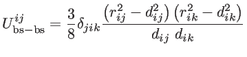 |
(2.21) |
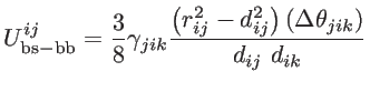 |
(2.22) |
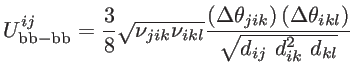 |
(2.23) |
where
 and
and
 are the non-equilibrium and equilibrium bond vectors from atom
to atom
are the non-equilibrium and equilibrium bond vectors from atom
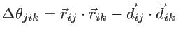
to atom  , respectively. The angle deviation of bonds between
and
, and
and
, respectively. The angle deviation of bonds between
and
, and
and  is defined by
 . The fitting parameters of silicon
  ,
,  ,
,  ,
,  , and
, and  are presented in Table 2.2 for both KVFF and MVFF models.
Table 2.2:
The force constant fitting parameters for silicon in
 .
.
| Model |
|
|
|
|
|
|---|
| KVFF [48] |
48.5 |
13.8 |
0 |
0 |
0 |
| MVFF [45] |
49.4 |
4.79 |
5.2 |
0.0 |
6.99 |
The total potential energy is zero when all the
atoms are located in their equilibrium position. Under the harmonic approximation, the
motion of atoms can be described by a dynamic matrix as:
![$\displaystyle D=\left[ D_{3\times 3}^{ij} \right]= \left[ \frac{1}{\sqrt{M_iM_j...
...\\ -\displaystyle \sum _{l\neq i}D_{il} & {,} & i=j \end{array} \right. \right]$](img221.png) |
(2.24) |
where dynamic matrix component between atoms
and
is given by [39]:
![$\displaystyle D_{ij}=\left[ \begin{array}{ccc} D_{ij}^{xx} & D_{ij}^{xy} & D_{i...
...y} & D_{ij}^{yz} \\ D_{ij}^{zx} & D_{ij}^{zy} & D_{ij}^{zz} \end{array} \right]$](img222.png) |
(2.25) |
and
![$\displaystyle D_{ij}^{mn}=\frac{\partial^2 U_{\mathrm{elastic}}}{\partial r_m^i \partial_n^j},~~~~~~ i,j\in N_{\mathrm{A}}~\mathrm{and}~m,n\in [x,y,z]$](img223.png) |
(2.26) |
is the second derivative of the potential energy with respect to the displacement of atom
along the  -axis and atom
along the
-axis and atom
along the  -axis.
 is
the potential associated with the motion of only two atoms
and
, whereas the
other atoms are considered frozen (unlike
is
the potential associated with the motion of only two atoms
and
, whereas the
other atoms are considered frozen (unlike  , which is the potential when all atoms are
allowed to move out of their equilibrium position). To compute
: 1) We start with
from Eq. 2.18. 2) We fix the positions of all atoms except atoms
and
. 3) We compute the inter-atomic potential due to all bond deformations that result from interaction between both of these two atoms, and sum them up to obtain
. All other inter-atomic potential terms that result from interactions due to atom
alone, or atom
alone, are not considered, since all double derivatives taken with respect to
, which is the potential when all atoms are
allowed to move out of their equilibrium position). To compute
: 1) We start with
from Eq. 2.18. 2) We fix the positions of all atoms except atoms
and
. 3) We compute the inter-atomic potential due to all bond deformations that result from interaction between both of these two atoms, and sum them up to obtain
. All other inter-atomic potential terms that result from interactions due to atom
alone, or atom
alone, are not considered, since all double derivatives taken with respect to
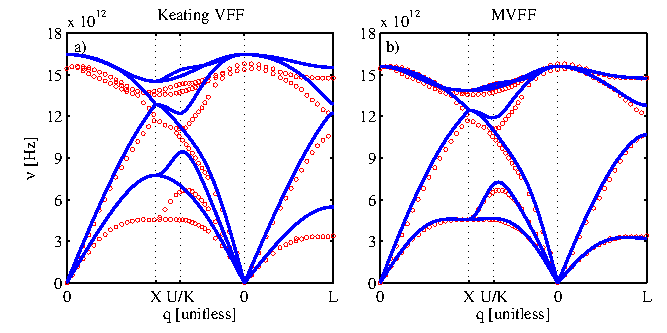
 , give zero. After setting up the dynamic matrix, the eigenvalue problem can be set up according to Eq. 2.12, the solution of which is the phononic dispersion. Figure 2.6 compares the bulk silicon dispersions calculated using the KVFF and MVFF models with experimental data taken from Ref. [49]. The KVFF fails in some part of the Brillouin zone, whereas the MVFF with three additional terms provides a more accurate description of the entire Brillouin zone.
Figure 2.6:
Phononic bandstructure of bulk silicon (solid) evaluated using (a) Keating VFF and (b) MVFF. Experimental results (circles) are taken from
Ref. [49].
|
|
Next: 2.3 Electron Transport
Up: 2.2 Silicon
Previous: 2.2.1 Electronic Structure
Contents
H. Karamitaheri: Thermal and Thermoelectric Properties of Nanostructures