The current density in the WFM is only constant, if the discrete formula for the calculation is chosen according to the discretization of the free operator. With the appropriate discretization the resulting current density comes out constant, now matter how crude the mesh is.
In Fig. 10.2 we depict the current density at the simulated
maximum bias of
![]() , if
we calculate it pointwise according to the ``naive'' formula
, if
we calculate it pointwise according to the ``naive'' formula
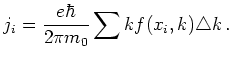 |
(10.1) |
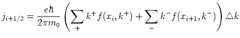 |
(10.2) |
Near the barriers the naive current density is far from constant and varies rapidly. Naive conservation of mass is severely violated and the current flows even backwards. It is seen that this property is very sensitive on the discretization as the mesh is too coarse. We note that for the I-V curves the current was calculated with the ``correct'' (conserved) formula.
![\includegraphics[width=0.9\columnwidth
]{Figures/jcompMax2}](img770.png)
|
![]()
![]()
![]()
![]() Previous: 10.1.1 I-V curves
Up: 10.1 Comparison of Simulation
Next: 10.1.3 Carrier Density
Previous: 10.1.1 I-V curves
Up: 10.1 Comparison of Simulation
Next: 10.1.3 Carrier Density