


 Previous: 2.1.2 Poisson Equation
Up: 2.1 The Boltzmann Poisson
Next: 2.1.4 Distribution Function Models
Previous: 2.1.2 Poisson Equation
Up: 2.1 The Boltzmann Poisson
Next: 2.1.4 Distribution Function Models
To derive a numerically tractable model from the full
(3+3)-dimensional Boltzmann equation we assume that
the distribution
 is
one-dimensional in space
is
one-dimensional in space
 and
has cylinder symmetry in
and
has cylinder symmetry in
 . That is
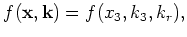 where where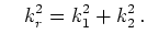 |
(2.11) |
This is known as the ``1+2''-Boltzmann equation.
Note that also the input data has to fulfill this symmetry.
Consequently the cylinder radial components of the
electrical field  vanish.
With this assumption we have
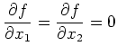 |
(2.12) |
and
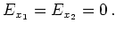 |
(2.13) |
Hence the BTE reduces for parabolic bands to
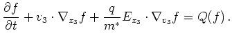 |
(2.14) |
Previous: 2.1.2 Poisson Equation
Up: 2.1 The Boltzmann Poisson
Next: 2.1.4 Distribution Function Models
R. Kosik: Numerical Challenges on the Road to NanoTCAD