2.2.1 Macroscopic Observables

For many TCAD purposes the kinetic description in terms of the distribution function $f(x,k)$ contains more information than is really needed and is numerically not tractable. The link to the continuum formulation is made by reducing the distribution to its first moments.

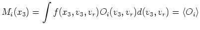
The macroscopic quantities (moments) $M(x)$ are the expectation values derived from the observables $O$ by integrating the distribution function $f$ over $k$-space with weight $O(k)$.

$$M_i(x_3) = \int f(x_3,v_3,v_r) O_i(v_3,v_r) d(v_3,v_r) = \langle O_i \rangle$$ (2.19)

In this equation $d(v_3,v_r)$ denotes the volume element stemming from the transformation to the new variables. (This is not given here explicitly as we never need it.) We denote the expectation value by $M = \langle O \rangle$.