In the desire to avoid interpolation from odd/even quantities to the even/odd grid (which we saw as an obstacle to reach convergence) the following idea for discretization was born: As we need the even quantities also on the odd grid why not simply add equations for the even quantities on the odd grid?
In this way we have two grids which are treated on a perfectly equal footing. If we need an even quantity on the odd grid no interpolation is involved, as the quantity is available from the equations for the second grid.
For illustration we give the equations for the fluxes.
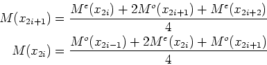
We now have two unknown quantities
![]() and
and
![]() and hence have two equations
and hence have two equations
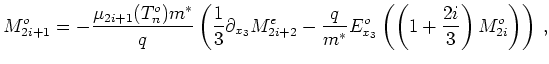 |
(4.1) |
 |
(4.2) |
We have Dirichlet boundary conditions for the even quantities. There are several ways to impose boundary conditions for the even quantities on the odd grid. The simplest is to use Dirichlet conditions too. The boundary value is then given by interpolation from the even grid. So interpolation is needed, but only for the boundary values.
Analysis of the resulting discretization shows that this does not avoid central differencing at all. If one views the two ``separated'' grids as one grid with the double number of points it can be seen that on the contrary the discretization applies central differencing consistently everywhere.
In practice for one quantity we get two distinct solution curves - one on the odd and one on the even grid. Both of these curves are smooth. We also get two constant lines for the current. In general the current values are different, hence an error estimate comes for free.
Such a result is depicted in Figure
4.1.
![\includegraphics[width=0.9\columnwidth]{Figures/current_cd2}](img248.png)
|
By refining the mesh we can check that the accuracy of the scheme is practically of second order on the used equi-spaced mesh. Doubling the number of mesh points means a reduction of the difference between the odd and even value of the current by a factor of four. By this property it is feasible to refine the grid until the difference is below a certain error bound.
Central-differencing artefacts in the solution can
be removed by post-processing. A simple ![]() interpolation
interpolation
 |
(4.3) |
removes them to a large extent and the solution curves look smooth.
When using the double grid discretization we also use two grids for the Poisson equation. Alternatively one can use a single big grid and combine this with the double grid discretization. This has the advantage that central difference effects are eliminated to a large extent. However, experiments show that we also lose the favorable convergence properties of the pure double grid discretization.
![]()
![]()
![]()
![]() Previous: 4.1.1 Variants of the
Up: 4.1 Discretization
Next: 4.1.3 Discussion
Previous: 4.1.1 Variants of the
Up: 4.1 Discretization
Next: 4.1.3 Discussion