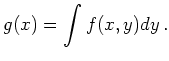
If ![]() and
and ![]() are random variables and
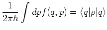
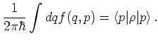
are random variables and ![]() is their joint probability
distribution, the marginal distribution
is their joint probability
distribution, the marginal distribution ![]() of
of ![]() is given by
is given by
 |
(6.54) |
| (6.55) |
 |
(6.56) |
 |
(6.57) |
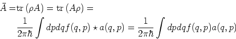
Classically the definition of the local (marginal) expectation
values
of observables is
not ambiguous due to the commutativity of all observables.
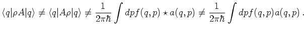
However, quantum mechanically to each way of calculating the expectation
value in 6.59 corresponds a definition for the local expectation
value ![]() and in general these definitions give different results
and in general these definitions give different results
 |
(6.59) |
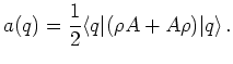
In general the operator ![]() is not selfadjoint, so the
definitions using Dirac brackets above are different.
We can rephrase this by using the
explicit expression for the density operator for
a pure state
is not selfadjoint, so the
definitions using Dirac brackets above are different.
We can rephrase this by using the
explicit expression for the density operator for
a pure state
![]() .
For a single wave function
.
For a single wave function ![]() we get two
definitions for the local expectation
we get two
definitions for the local expectation ![]()
| (6.60) |
A good way to define the local expectation is to symmetrize the definitions
This definition has the property that
![]() is
again a selfadjoint operator,
hence the local expectation is real. This is the
way in which the current
is
again a selfadjoint operator,
hence the local expectation is real. This is the
way in which the current ![]() is conventionally defined.
is conventionally defined.
A special case which is not treated in this way
is the definition of local expectation for
an energy-like operator ![]() where
where ![]() is selfadjoint.
Then we can define
is selfadjoint.
Then we can define
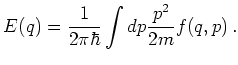
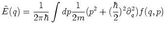
However, in the Wigner formalism one usually defines energy
as the second
![]() -moment in the form
-moment in the form
With this definition for the local expectation value the
local energy ![]() can become negative, as was observed in
Wigner function simulations.
can become negative, as was observed in
Wigner function simulations.
To calculate the Wigner transformation of
![]() we use a suitable definition
for the star product.
We get
we use a suitable definition
for the star product.
We get
 |
(6.64) |
The question of marginalization is also discussed in [Wlo99].
![]()
![]()
![]()
![]() Previous: 6.2.4 Probabilistic Structure
Up: 6.2 Quantum Mechanics in
Next: 6.2.6 A Feasible Phase
Previous: 6.2.4 Probabilistic Structure
Up: 6.2 Quantum Mechanics in
Next: 6.2.6 A Feasible Phase